Download presentation
Presentation is loading. Please wait.

1
Microarray data analysis David A. McClellan, Ph.D. Introduction to Bioinformatics david_mcclellan@byu.edu Brigham Young University Dept. Integrative Biology 25 January 2006

2
Inferential statistics Inferential statistics are used to make inferences about a population from a sample. Hypothesis testing is a common form of inferential statistics. A null hypothesis is stated, such as: “There is no difference in signal intensity for the gene expression measurements in normal and diseased samples.” The alternative hypothesis is that there is a difference. We use a test statistic to decide whether to accept or reject the null hypothesis. For many applications, we set the significance level to p < 0.05. Page 199

3
Inferential statistics A t-test is a commonly used test statistic to assess the difference in mean values between two groups. t = = Questions Is the sample size (n) adequate? Are the data normally distributed? Is the variance of the data known? Is the variance the same in the two groups? Is it appropriate to set the significance level to p < 0.05? Page 199 x 1 – x 2 difference between mean values variability (noise)
 adequate. Are the data normally distributed. Is the variance of the data known. Is the variance the same in the two groups. Is it appropriate to set the significance level to p < Page 199 x 1 – x 2 difference between mean values variability (noise).")
4
Inferential statistics ParadigmParametric testNonparametric Compare two unpaired groupsUnpaired t-testMann-Whitney test Compare two paired groupsPaired t-testWilcoxon test Compare 3 orANOVA more groups Page 198-200

5
ANOVA ANalysis Of VAriance ANOVA calculates the probability that several conditions all come from the same distribution

6
Parametric vs. Nonparametric Parametric tests are applied to data sets that are sampled from a normal distribution (t- tests & ANOVAs) Nonparametric tests do not make assumptions about the population distribution – they rank the outcome variable from low to high and analyze the ranks
 Nonparametric tests do not make assumptions about the population distribution – they rank the outcome variable from low to high and analyze the ranks.")
7
Mann-Whitney test (a two-sample rank test) Actual measurements are not employed; the ranks of the measurements are used instead n 1 and n 2 are the number of observations in samples 1 and 2, and R 1 is the sum of the ranks of the observations in sample 1
 Actual measurements are not employed; the ranks of the measurements are used instead n 1 and n 2 are the number of observations in samples 1 and 2, and R 1 is the sum of the ranks of the observations in sample 1")
8
Mann-Whitney example

9
Mann-Whitney table

10
Wilcoxon paired-sample test A nonparametric analogue to the paired- sample t-test, just as the Mann-Whitney test is a nonparametric procedure analogous to the unpaired-sample t-test

11
Wilcoxon example

12
Wilcoxon table

13
Inferential statistics Is it appropriate to set the significance level to p < 0.05? If you hypothesize that a specific gene is up-regulated, you can set the probability value to 0.05. You might measure the expression of 10,000 genes and hope that any of them are up- or down-regulated. But you can expect to see 5% (500 genes) regulated at the p < 0.05 level by chance alone. To account for the thousands of repeated measurements you are making, some researchers apply a Bonferroni correction. The level for statistical significance is divided by the number of measurements, e.g. the criterion becomes: p < (0.05)/10,000 or p < 5 x 10 -6 Page 199
 regulated at the p < 0.05 level by chance alone. To account for the thousands of repeated measurements you are making, some researchers apply a Bonferroni correction. The level for statistical significance is divided by the number of measurements, e.g. the criterion becomes: p < (0.05)/10,000 or p < 5 x Page 199.")
14
Page 200 Significance analysis of microarrays (SAM) SAM-- an Excel plug-in -- URL: www-stat.stanford.edu/~tibs/SAM -- modified t-test -- adjustable false discovery rate
 SAM-- an Excel plug-in -- URL: www-stat.stanford.edu/~tibs/SAM -- modified t-test -- adjustable false discovery rate")
15
Page 202

16
up- regulated Page 202 down- regulated expected observed

17
Descriptive statistics Microarray data are highly dimensional: there are many thousands of measurements made from a small number of samples. Descriptive (exploratory) statistics help you to find meaningful patterns in the data. A first step is to arrange the data in a matrix. Next, use a distance metric to define the relatedness of the different data points. Two commonly used distance metrics are: -- Euclidean distance -- Pearson coefficient of correlation 203
 statistics help you to find meaningful patterns in the data. A first step is to arrange the data in a matrix. Next, use a distance metric to define the relatedness of the different data points. Two commonly used distance metrics are: -- Euclidean distance -- Pearson coefficient of correlation 203.")
18
Euclidean Distance

19
Pearson Correlation Coefficient

20
Descriptive statistics: clustering Clustering algorithms offer useful visual descriptions of microarray data. Genes may be clustered, or samples, or both. We will next describe hierarchical clustering. This may be agglomerative (building up the branches of a tree, beginning with the two most closely related objects) or divisive (building the tree by finding the most dissimilar objects first). In each case, we end up with a tree having branches and nodes. Page 204
 or divisive (building the tree by finding the most dissimilar objects first). In each case, we end up with a tree having branches and nodes. Page 204.")
21
Agglomerative clustering a b c d e a,b 43210 Page 206

22
a b c d e a,b d,e 43210 Agglomerative clustering Page 206

23
a b c d e a,b d,e c,d,e 43210 Agglomerative clustering Page 206

24
a b c d e a,b d,e c,d,e a,b,c,d,e 43210 Agglomerative clustering …tree is constructed Page 206

25
Divisive clustering a,b,c,d,e 43210 Page 206

26
Divisive clustering c,d,e a,b,c,d,e 43210 Page 206

27
Divisive clustering d,e c,d,e a,b,c,d,e 43210 Page 206

28
Divisive clustering a,b d,e c,d,e a,b,c,d,e 43210 Page 206

29
Divisive clustering a b c d e a,b d,e c,d,e a,b,c,d,e 43210 …tree is constructed Page 206

30
divisive agglomerative a b c d e a,b d,e c,d,e a,b,c,d,e 43210 43210 Page 206

31
1 12 1 Page 207

32
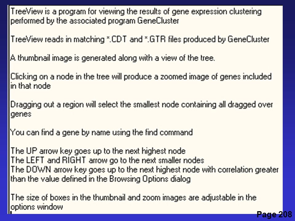
Cluster and TreeView Page 208

33
Cluster and TreeView clustering PCASOMK means Page 208

34
Cluster and TreeView Page 208

35
Cluster and TreeView Page 208

39
Page 209 Two-way clustering of genes (y-axis) and cell lines (x-axis) (Alizadeh et al., 2000)
 and cell lines (x-axis) (Alizadeh et al., 2000)")
40
Self-Organizing Maps (SOM) To download GeneCluster: http://www.genome.wi.mit.edu/MPR/software.html
 To download GeneCluster:")
41
Page 211 SOMs are unsupervised neural net algorithms that identify coregulated genes

42
Two pre-processing steps essential to apply SOMs 1. Variation Filtering: Data are passed through a variation filter to eliminate those genes showing no significant change in expression across the k samples. This step is needed to prevent nodes from being attracted to large sets of invariant genes. 2. Normalization: The expression level of each gene is normalized across experiments. This focuses attention on the 'shape' of expression patterns rather than absolute levels of expression.

43
An exploratory technique used to reduce the dimensionality of the data set to 2D or 3D For a matrix of m genes x n samples, create a new covariance matrix of size n x n Thus transform some large number of variables into a smaller number of uncorrelated variables called principal components (PCs). Principal components analysis (PCA) Page 211
 Page 211.")
44
Principal component axis #2 (10%) Principal component axis #1 (87%) PC#3: 1% C3 C4 C2 C1 N2 N3 N4 P1 P4 P2 P3 Lead (P) Sodium (N) Control (C) Legend Principal components analysis (PCA), an exploratory technique that reduces data dimensionality, distinguishes lead-exposed from control cell lines
 Principal component axis #1 (87%) PC#3: 1% C3 C4 C2 C1 N2 N3 N4 P1 P4 P2 P3 Lead (P) Sodium (N) Control (C) Legend Principal components analysis (PCA), an exploratory technique that reduces data dimensionality, distinguishes lead-exposed from control cell lines")
45
Principal components analysis (PCA): objectives to reduce dimensionality to determine the linear combination of variables to choose the most useful variables (features) to visualize multidimensional data to identify groups of objects (e.g. genes/samples) to identify outliers Page 211
 to identify outliers Page 211.")
46
Page 212 http://www.okstate.edu/artsci/botany/ordinate/PCA.htm

47
Page 212 http://www.okstate.edu/artsci/botany/ordinate/PCA.htm

48
Page 212

49
Chr 21 Use of PCA to demonstrate increased levels of gene expression from Down syndrome (trisomy 21) brain
 brain")
Similar presentations


 for Clustering Gene Expression Data K. Y. Yeung and W. L. Ruzzo.>")


843-6015 E-mail:>")


 Allows study of thousands of genes at.>")


