2. Overview Part 1 - Storage Elements and Analysis
Introduction to sequential circuits
Types of sequential circuits
Storage elements
Latches
Flip-flops
Sequential circuit analysis
State tables
State diagrams
Circuit and System Timing
Part 2 - Sequential Circuit Design
Specification
Assignment of State Codes
Implementation

3. Introduction to Sequential Circuits
Inputs
Outputs
Combina-tional
Logic
A Sequential circuit contains:
Storage elements: Latches or Flip-Flops
Combinatorial Logic:
Implements a multiple-output switching function
Inputs are signals from the outside.
Outputs are signals to the outside.
Other inputs, State or Present State, are signals from storage elements.
The remaining outputs, Next State are inputs to storage elements.
Storage Elements
State
Next
State

4. Introduction to Sequential Circuits
Combinatorial Logic
Next state function Next State = f(Inputs, State)
Output function (Mealy) Outputs = g(Inputs, State)
Output function (Moore) Outputs = h(State)
Output function type depends on specification and affects the design significantly
Inputs
Outputs
Combina-tional
Logic
Storage Elements
State
Next
State

5. Types of Sequential Circuits
Depends on the times at which:
storage elements observe their inputs, and
storage elements change their state
Synchronous
Behavior defined from knowledge of its signals at discrete instances of time
Storage elements observe inputs and can change state only in relation to a timing signal (clock pulses from a clock)
Asynchronous
Behavior defined from knowledge of inputs an any instant of time and the order in continuous time in which inputs change
If clock just regarded as another input, all circuits are asynchronous!
Nevertheless, the synchronous abstraction makes complex designs tractable!

6. Discrete Event Simulation
In order to understand the time behavior of a sequential circuit we use discrete event simulation.
Rules:
Gates modeled by an ideal (instantaneous) function and a fixed gate delay
Any change in input values is evaluated to see if it causes a change in output value
Changes in output values are scheduled for the fixed gate delay after the input change
At the time for a scheduled output change, the output value is changed along with any inputs it drives

7. Simulated NAND Gate Example: A 2-Input NAND gate with a 0.5 ns. delay:
Assume A and B have been 1 for a long time
At time t=0, A changes to a 0 at t= 0.8 ns, back to 1. F A B
DELAY 0.5 ns.
F(Instantaneous)
t (ns) A B
F(I) F
Comment –  1
A=B=1 for a long time Þ Ü
F(I) changes to 1
0.5
F changes to 1 after a 0.5 ns delay
0.8
F(Instantaneous) changes to 0
0.13
F changes to 0 after a 0.5 ns delay

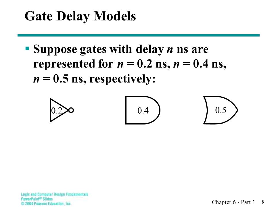
8. Gate Delay Models
Suppose gates with delay n ns are represented for n = 0.2 ns, n = 0.4 ns, n = 0.5 ns, respectively:
0.2
0.5
0.4

9. Circuit Delay Model A Y S B A B S Y
Consider a simple input multiplexer:
With function:
Y = A for S = 1
Y = B for S = 0
“Glitch” is due to delay of inverter
0.4
0.2
0.5 Y S
0.4 B A S B Y

10. Storing State S Y B B S Y What if A con- nected to Y? Circuit becomes:
With function:
Y = B for S = 1, and Y(t) dependent on Y(t – 0.9) for S = 0
The simple combinational circuit has now become a sequential circuit because its output is a function of a time sequence of input signals! S B Y
0.5
0.4
0.2 B S Y
Y is stored value in shaded area

11. Storing State (Continued)
Simulation example as input signals change with time. Changes occur every 100 ns, so that the tenths of ns delays are negligible.
Y represent the state of the circuit, not just an output.  
Time B S Y
Comment 1
Y “remembers” 0
Y = B when S = 1
Now Y “remembers” B = 1 for S = 0
No change in Y when B changes
Y “remembers” B = 0 for S = 0
Note that the “glitch” is still present. An actual storage circuit would be designed to eliminate this by addition of term BY.

12. Storing State (Continued)
Suppose we place an inverter in the “feedback path.”
The following behavior results:
The circuit is said to be unstable.
For S = 0, the circuit has become what is called an oscillator. Can be used as crude clock. S B Y
0.2
0.5
0.4 B S Y
Comment 1
Y = B when S = 1
Now Y “remembers” A Y,
1.1 ns later
Y, 1.1 ns later

13. Basic (NAND) S – R Latch
“Cross-Coupling” two NAND gates gives the S -R Latch:
Which has the time sequence behavior:
S = 0, R = 0 is forbidden as input pattern
S (set) Q Q
R (reset)
Time R S Q
Comment 1 ?
Stored state unknown
“Set” Q to 1
Now Q “remembers” 1
“Reset” Q to 0 1 1 1
Now Q “remembers” 0 1 1
Both go high 1 1 ? ?
Unstable!

14. Basic (NOR) S – R Latch
Cross-coupling two NOR gates gives the S – R Latch:
Which has the time sequence behavior:
S (set)
R (reset) Q R S Q
Comment ?
Stored state unknown 1
“Set” Q to 1
Now Q “remembers” 1
“Reset” Q to 0
Now Q “remembers” 0
Both go low
Unstable!
Time

15. Clocked S - R Latch
Adding two NAND gates to the basic S - R NAND latch gives the clocked S – R latch:
Has a time sequence behavior similar to the basic S-R latch except that the S and R inputs are only observed when the line C is high.
C means “control” or “clock”. S R Q C

16. Clocked S - R Latch (continued)
The Clocked S-R Latch can be described by a table:
The table describes what happens after the clock [at time (t+1)] based on:
current inputs (S,R) and
current state Q(t). S R Q C

17. D Latch Adding an inverter to the S-R Latch, gives the D Latch:
Note that there are no “indeterminate” states! D Q C Q D
Q(t+1)
Comment
No change 1
Set Q
Clear Q
No Change C D Q

18. Flip-Flops The latch timing problem Master-slave flip-flop
Edge-triggered flip-flop
Standard symbols for storage elements
Direct inputs to flip-flops
Flip-flop timing

19. The Latch Timing Problem
In a sequential circuit, paths may exist through combinational logic:
From one storage element to another
From a storage element back to the same storage element
The combinational logic between a latch output and a latch input may be as simple as an interconnect
For a clocked D-latch, the output Q depends on the input D whenever the clock input C has value 1

20. The Latch Timing Problem (continued)
Consider the following circuit:
Suppose that initially Y = 0.
As long as C = 1, the value of Y continues to change!
The changes are based on the delay present on the loop through the connection from Y back to Y.
This behavior is clearly unacceptable.
Desired behavior: Y changes only once per clock pulse C D Q Y
Clock
Clock Y

21. The Latch Timing Problem (continued)
A solution to the latch timing problem is to break the closed path from Y to Y within the storage element
The commonly-used, path-breaking solutions replace the clocked D-latch with:
a master-slave flip-flop
an edge-triggered flip-flop

22. S-R Master-Slave Flip-Flop
Consists of two clocked S-R latches in series with the clock on the second latch inverted
The input is observed by the first latch with C = 1
The output is changed by the second latch with C = 0
The path from input to output is broken by the difference in clocking values (C = 1 and C = 0).
The behavior demonstrated by the example with D driven by Y given previously is prevented since the clock must change from 1 to 0 before a change in Y based on D can occur. C S R Q

23. Flip-Flop Problem
The change in the flip-flop output is delayed by the pulse width which makes the circuit slower or
S and/or R are permitted to change while C = 1
Suppose Q = 0 and S goes to 1 and then back to 0 with R remaining at 0
The master latch sets to 1
A 1 is transferred to the slave
Suppose Q = 0 and S goes to 1 and back to 0 and R goes to 1 and back to 0
The master latch sets and then resets
A 0 is transferred to the slave
This behavior is called 1s catching

24. Flip-Flop Solution Use edge-triggering instead of master-slave
An edge-triggered flip-flop ignores the pulse while it is at a constant level and triggers only during a transition of the clock signal
Edge-triggered flip-flops can be built directly at the electronic circuit level, or
A master-slave D flip-flop which also exhibits edge-triggered behavior can be used.

25. Edge-Triggered D Flip-Flop
The edge-triggered D flip-flop is the same as the master- slave D flip-flop
It can be formed by:
Replacing the first clocked S-R latch with a clocked D latch or
Adding a D input and inverter to a master-slave S-R flip-flop
The delay of the S-R master-slave flip-flop can be avoided since the 1s-catching behavior is not present with D replacing S and R inputs
The change of the D flip-flop output is associated with the negative edge at the end of the pulse
It is called a negative-edge triggered flip-flop C S R Q D

26. Positive-Edge Triggered D Flip-Flop
Formed by adding inverter to clock input
Q changes to the value on D applied at the positive clock edge within timing constraints to be specified
Our choice as the standard flip-flop for most sequential circuits C S R Q D

27. Standard Symbols for Storage Elements
Master-Slave: Postponed output indicators
Edge-Triggered: Dynamic indicator
(a) Latches S R SR
D with 0 Control D C
D with 1 Control
(b) Master-Slave Flip-Flops
Triggered D
Triggered SR
(c) Edge-Triggered Flip-Flops

28. Direct Inputs
At power up or at reset, all or part of a sequential circuit usually is initialized to a known state before it begins operation
This initialization is often done outside of the clocked behavior of the circuit, i.e., asynchronously.
Direct R and/or S inputs that control the state of the latches within the flip-flops are used for this initialization.
For the example flip-flop shown
0 applied to R resets the flip-flop to the 0 state
0 applied to S sets the flip-flop to the 1 state D C S R Q

29. Flip-Flop Timing Parameters
ts - setup time
th - hold time
tw - clock pulse width
tpx - propa- gation delay
tPHL - High-to- Low
tPLH - Low-to- High
tpd - max (tPHL, tPLH) t $ t wH
wH,min C t $ t wL
wL,min t t s h S / R t
p-,min t
p-,max Q
(a) Pulse-triggered (positive pulse) t $ t wH
wH,min C t $ t wL
wL,min t t s h D t
p-,min t
p-,max Q
(b) Edge-triggered (negative edge)

30. Flip-Flop Timing Parameters (continued)
ts - setup time
Master-slave - Equal to the width of the triggering pulse
Edge-triggered - Equal to a time interval that is generally much less than the width of the the triggering pulse
th - hold time - Often equal to zero
tpx - propagation delay
Same parameters as for gates except
Measured from clock edge that triggers the output change to the output change

31. Sequential Circuit Analysis
General Model
Current State at time (t) is stored in an array of flip-flops. 
Next State at time (t+1) is a Boolean function of State and Inputs.
Outputs at time (t) are a Boolean function of State (t) and (sometimes) Inputs (t).
Inputs
Combina-tional
Logic
Outputs
Storage Elements
CLK
State
Next
State

32. Example 1 (from Fig. 6-17) Input: x(t) Output: y(t)
State: (A(t), B(t))
What is the Output Function?
What is the Next State Function? A C D Q y x B CP

33. Example 1 (from Fig. 6-17) (continued)
Boolean equations for the functions:
A(t+1) = A(t)x(t) B(t)x(t)
B(t+1) = A(t)x(t)
y(t) = x(t)(B(t) + A(t)) x D Q A C Q A
Next State D Q B CP C Q' y
Output

34. Example 1(from Fig. 6-17) (continued)
Where in time are inputs, outputs and states defined? 1

35. State Table Characteristics
State table – a multiple variable table with the following four sections:
Present State – the values of the state variables for each allowed state.
Input – the input combinations allowed.
Next-state – the value of the state at time (t+1) based on the present state and the input.
Output – the value of the output as a function of the present state and (sometimes) the input.
From the viewpoint of a truth table:
the inputs are Input, Present State
and the outputs are Output, Next State

36. Example 1: State Table (from Fig. 6-17)
The state table can be filled in using the next state and output equations: A(t+1) = A(t)x(t) + B(t)x(t) B(t+1) =A (t)x(t) y(t) =x (t)(B(t) + A(t))
Present State
Input
Next State
Output
A(t) B(t)
x(t)
A(t+1) B(t+1)
y(t) 1

37. Example 1: Alternate State Table
2-dimensional table that matches well to a K-map. Present state rows and input columns in Gray code order.
A(t+1) = A(t)x(t) + B(t)x(t)
B(t+1) =A (t)x(t)
y(t) =x (t)(B(t) + A(t))
Present
State
Next State
x(t)= x(t)=1
Output
x(t)=0 x(t)=1
A(t) B(t)
A(t+1)B(t+1) A(t+1)B(t+1)
y(t) y(t)
0 0
0 1
1 0
1 1

38. State Diagrams
The sequential circuit function can be represented in graphical form as a state diagram with the following components:
A circle with the state name in it for each state
A directed arc from the Present State to the Next State for each state transition
A label on each directed arc with the Input values which causes the state transition, and
A label:
On each circle with the output value produced, or
On each directed arc with the output value produced.

39. State Diagrams Label form: On circle with output included:
state/output
Moore type output depends only on state
On directed arc with the output included:
input/output
Mealy type output depends on state and input

40. Example 1: State Diagram
A B
0 0
0 1
1 1
1 0
x=0/y=1
x=1/y=0
x=0/y=0
Which type?
Diagram gets confusing for large circuits
For small circuits, usually easier to understand than the state table
Type: Mealy

41. Moore and Mealy Models
Sequential Circuits or Sequential Machines are also called Finite State Machines (FSMs). Two formal models exist:
In contemporary design, models are sometimes mixed Moore and Mealy
Moore Model
Named after E.F. Moore.
Outputs are a function ONLY of states
Usually specified on the states.
Mealy Model
Named after G. Mealy
Outputs are a function of inputs AND states
Usually specified on the state transition arcs.

42. Moore and Mealy Example Diagrams
Mealy Model State Diagram maps inputs and state to outputs
Moore Model State Diagram maps states to outputs 1
x=1/y=1
x=1/y=0
x=0/y=0
1/0
2/1
x=1
x=0
0/0

43. Moore and Mealy Example Tables
Mealy Model state table maps inputs and state to outputs
Moore Model state table maps state to outputs
Present
State
Next State
x=0 x=1
Output 1
Present
State
Next State
x=0 x=1
Output 1 2

44. Example 2: Sequential Circuit Analysis
Clock
Reset D Q C R A B Z
Logic Diagram:

45. Example 2: Flip-Flop Input Equations
Variables
Inputs: None
Outputs: Z
State Variables: A, B, C
Initialization: Reset to (0,0,0)
Equations
A(t+1) = Z =
B(t+1) =
C(t+1) =
A(t+1) = BC
B(t+1) = B’C + BC’
C(t+1) = A’C’
Z = A

46. Example 2: State Table X’ = X(t+1) A B C A’B’C’ Z 0 0 0 0 0 1 0 1 0
A’B’C’: , , , , , , , Z:

47. Example 2: State Diagram
Which states are used?
What is the function of the circuit?
000
011
010
001
100
101
110
111
Reset
ABC
Only states reachable from the reset state 000 are used: 000, 001, 010, 011, and 100.
The circuit produces a 1 on Z after four clock periods and every five clock periods thereafter:
000 -> 001 -> 010 -> 011 -> 100 -> 000 -> 001 -> 010 -> 011 -> 100 …

48. Circuit and System Level Timing
Consider a system comprised of ranks of flip-flops connected by logic:
If the clock period is too short, some data changes will not propagate through the circuit to flip-flop inputs before the setup time interval begins C D Q Q'
CLOCK

49. Circuit and System Level Timing (continued)
Timing components along a path from flip-flop to flip-flop
(a) Edge-triggered (positive edge) t p
pd,FF
pd,COMB
slack s C
(b) Pulse-triggered (negative pulse)

50. Circuit and System Level Timing (continued)
New Timing Components
tp - clock period - The interval between occurrences of a specific clock edge in a periodic clock
tpd,COMB - total delay of combinational logic along the path from flip-flop output to flip-flop input
tslack - extra time in the clock period in addition to the sum of the delays and setup time on a path
Can be either positive or negative
Must be greater than or equal to zero on all paths for correct operation

51. Circuit and System Level Timing (continued)
Timing Equations tp = tslack + (tpd,FF + tpd,COMB + ts)
For tslack greater than or equal to zero, tp ≥ max (tpd,FF + tpd,COMB + ts) for all paths from flip-flop output to flip-flop input
Can be calculated more precisely by using tPHL and tPLH values instead of tpd values, but requires consideration of inversions on paths

52. Calculation of Allowable tpd,COMB
Compare the allowable combinational delay for a specific circuit: a) Using edge-triggered flip-flops b) Using master-slave flip-flops
Parameters
tpd,FF(max) = 1.0 ns
ts(max) = 0.3 ns for edge-triggered flip-flops
ts = twH = 1.0 ns for master-slave flip-flops
Clock frequency = 250 MHz

53. Calculation of Allowable tpd,COMB (continued)
Calculations: tp = 1/clock frequency = 4.0 ns
Edge-triggered: 4.0 ≥ tpd,COMB + 0.3, tpd,COMB ≤ 2.7 ns
Master-slave: 4.0 ≥ tpd,COMB + 1.0, tpd,COMB ≤ 2.0 ns
Comparison: Suppose that for a gate, average tpd = 0.3 ns
Edge-triggered: Approximately 9 gates allowed on a path
Master-slave: Approximately 6 to 7 gates allowed on a path

54. Terms of Use © 2004 by Pearson Education,Inc. All rights reserved.
The following terms of use apply in addition to the standard Pearson Education Legal Notice.
Permission is given to incorporate these materials into classroom presentations and handouts only to instructors adopting Logic and Computer Design Fundamentals as the course text.
Permission is granted to the instructors adopting the book to post these materials on a protected website or protected ftp site in original or modified form. All other website or ftp postings, including those offering the materials for a fee, are prohibited.
You may not remove or in any way alter this Terms of Use notice or any trademark, copyright, or other proprietary notice, including the copyright watermark on each slide.
Return to Title Page