2. DREAM PLAN IDEA IMPLEMENTATION 1

3. 2

4. 3 Introduction to Image Processing Dr. Kourosh Kiani Email: kkiani2004@yahoo.comkkiani2004@yahoo.com Email: Kourosh.kiani@aut.ac.irKourosh.kiani@aut.ac.ir Email: Kourosh.kiani@semnan.ac.irKourosh.kiani@semnan.ac.ir Web: www.kouroshkiani.comwww.kouroshkiani.com Present to: Amirkabir University of Technology (Tehran Polytechnic) & Semnan University

5. Lecture 10 4 2D Discrete Fourier Transform (DFT)

6.  The two-dimensional Fourier transform and its inverse  Fourier transform (discrete case) DFt  Inverse Fourier transform:  u, v : the transform or frequency variables  x, y : the spatial or image variables

7. DFT -6.80 + 7.89i 17.8 - 12.76i17.8 -7.89i -6.8 - 7.89i103.00 19.28 + 9.2i 2.05+ 20.34i5.07 - 13.76i -5.09+- 13.76i9.28-10.82i 8.43 + 1.31i9.22 + 14.89i 6.09 + 3.25i-3.55 +13.88i-0.78+ 8i -3.55 – 13.88i6.09 - 3.25i9.22 - 14.89i8.43 - 1.31i-0.78+ 8i -5.09 + 13.76i5.07 + 2.13i2.05 - 1.83i19.28 - 9.2i 9.28-10.82i

8. 103.0010.4121.90 10.41 14.2614.675.5020.4421.36 8.0414.336.9017.518.53 8.048.5317.516.9014.33 14.2621.3620.445.5014.67 |F|=abs(F)= 2.011.021.34 1.02 1.151.170.741.311.33 0.911.160.841.240.93 0.910.931.240.841.16 1.151.331.310.741.17 log 10 |F|=log 10 (abs(F)) =

9. 0.00- 2.28-0.620.622.28 -0.861.93-0.401.470.45 -1.671.820.491.020.15 1.67-0.15-1.02 -0.49-1.82 0.86-0.45-1.470.40-1.93 angleF = 0.00- 130.76- 5.6435.64130.76 -49.39110.30- 2.7484.2625.51 - 95.57104.3328.0858.238.86 95.57- 8.8658.23--28.08- 04.33 49.39 -25.51 - 84.2622.74110.30- radToDegF=

11. Inverse Fourier transform -6.80 + 7.89i 17.8 - 12.76i17.8 -7.89i -6.8 - 7.89i103.00 19.28 + 9.2i 2.05+ 20.34i5.07 - 13.76i -5.09+- 13.76i9.28-10.82i 8.43 + 1.31i9.22 + 14.89i 6.09 + 3.25i-3.55 +13.88i-0.78+ 8i -3.55 – 13.88i6.09 - 3.25i9.22 - 14.89i8.43 - 1.31i-0.78+ 8i -5.09 + 13.76i5.07 + 2.13i2.05 - 1.83i19.28 - 9.2i 9.28-10.82i

12. Inverse Fourier transform

13. Magnitude and Phase of DFT What is more important? magnitude phase

14. Magnitude and Phase of DFT Reconstructed image using magnitude only Reconstructed image using phase only

15. original amplitude phase Magnitude and Phase of DFT

16. Example: DFT of 2D rectangle function Fourier spectrum Input function Spectrum displayed as an intensity function

17. Extending DFT to 2D 2D cos/sin functions

18. 2D - DFT Base-functions are waves u v

24. Why is DFT Useful? Easier to remove undesirable frequencies. Faster perform certain operations in the frequency domain than in the spatial domain.

25. Properties in the frequency domain Fourier transform works globally – No direct relationship between a specific components in an image and frequencies Intuition about frequency – Frequency content – Rate of change of gray levels in an image

26. Example: Removing undesirable frequencies remove high frequencies reconstructed signal frequencies noisy signal To remove certain frequencies, set their corresponding F(u) coefficients to zero!

27. How do frequencies show up in an Signal? Low frequencies correspond to slowly varying information High frequencies correspond to quickly varying information

28. How do frequencies show up in an image? Low frequencies correspond to slowly varying information (e.g., continuous surface). High frequencies correspond to quickly varying information (e.g., edges)

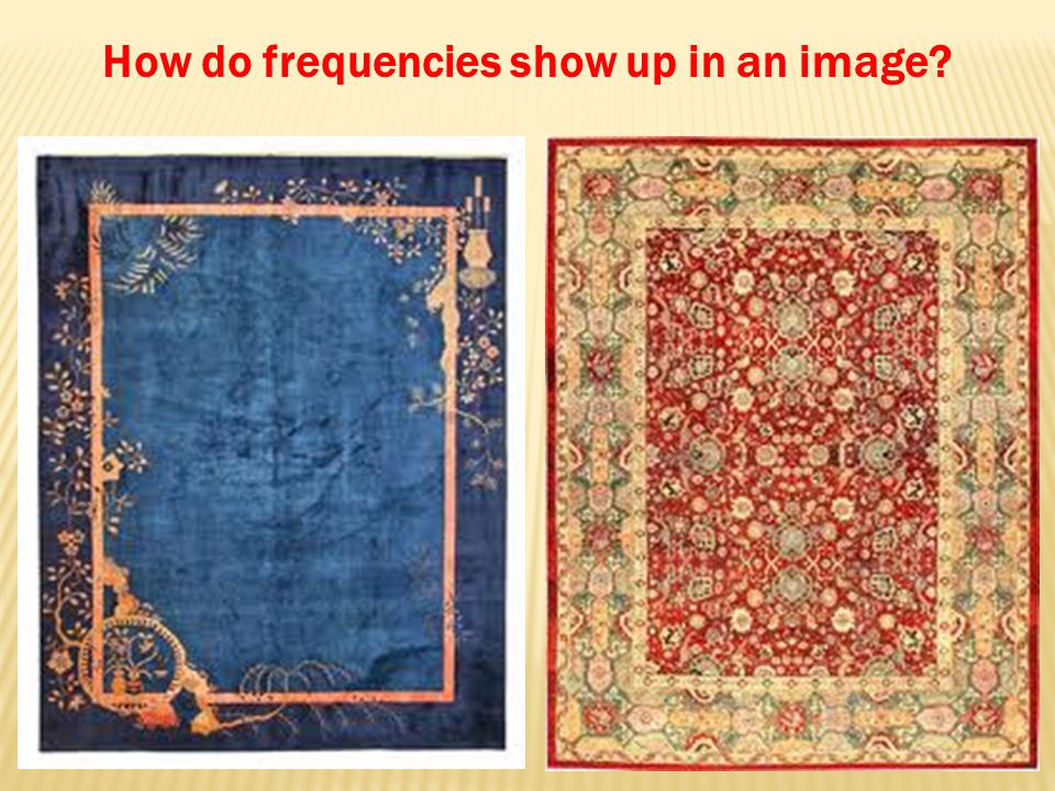
29. How do frequencies show up in an image?

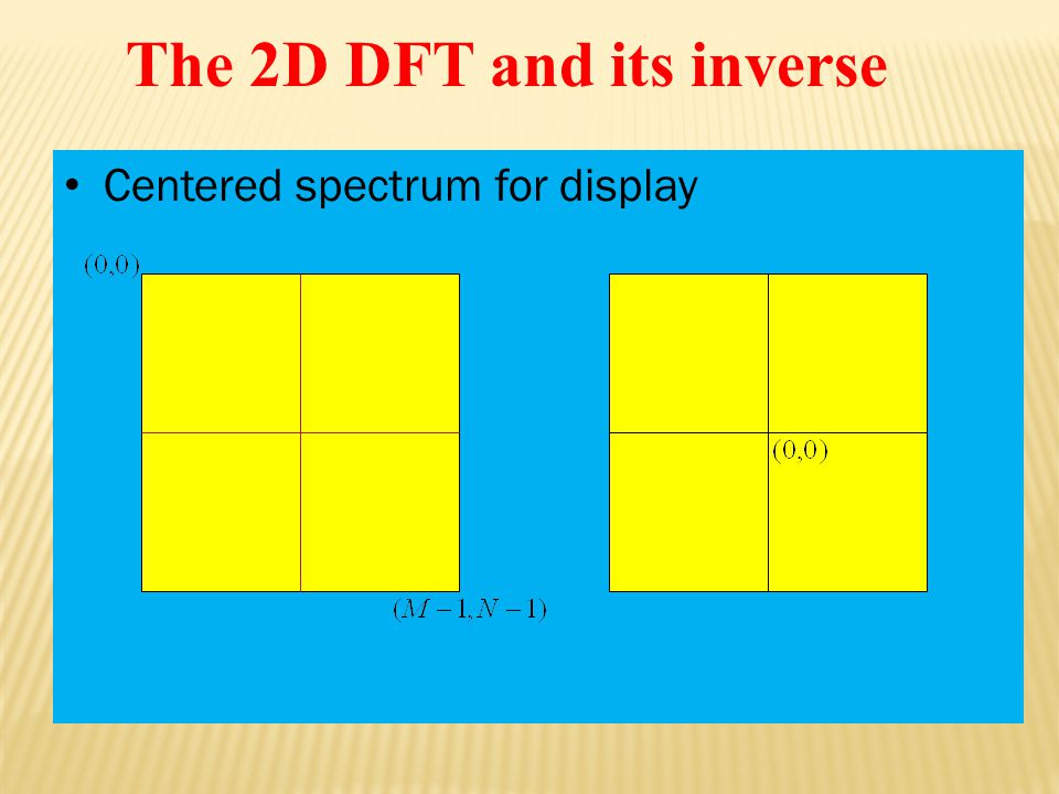
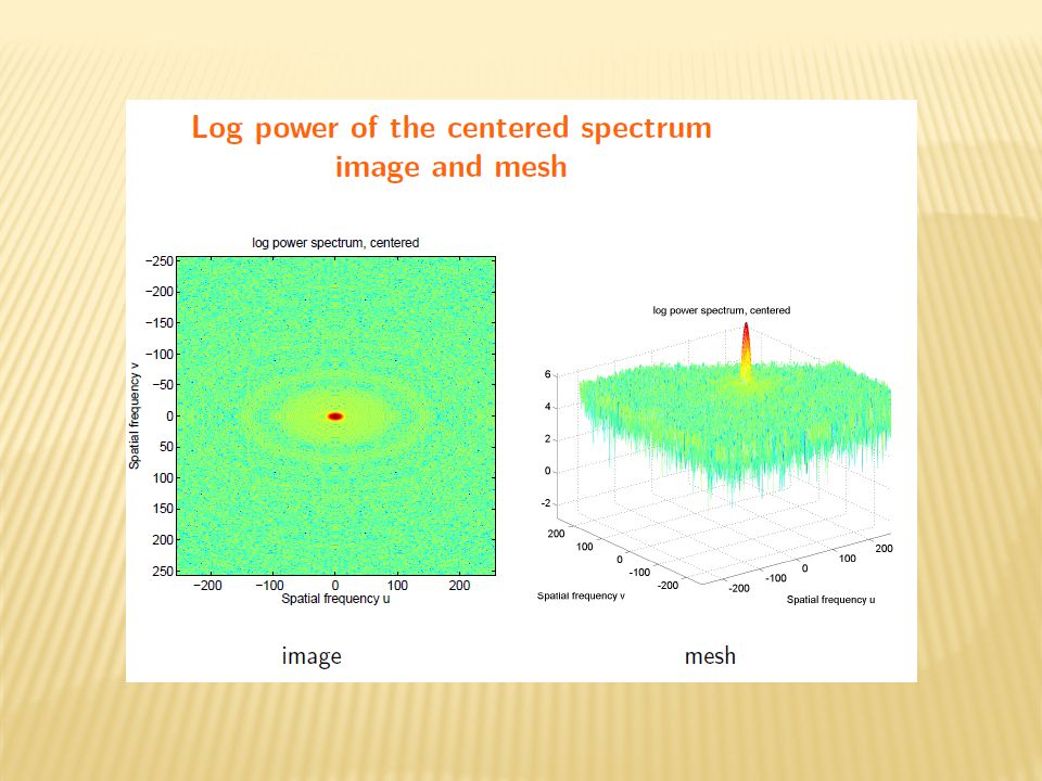
36. The 2D DFT and its inverse Centered spectrum for display

37. 2-D Fourier transform Frequency axis x y u v u v Fshift 0

47. Low and high frequencies Low High Low High Low High Frequencies of the 2D DFT

48. Periodicity of 2-D DFT For an image of size NxM pixels, its 2-D DFT repeats itself every N points in x- direction and every M points in y-direction. We display only in this range 0N2N-N 0 M 2M -M 2-D DFT: f(x,y)f(x,y)

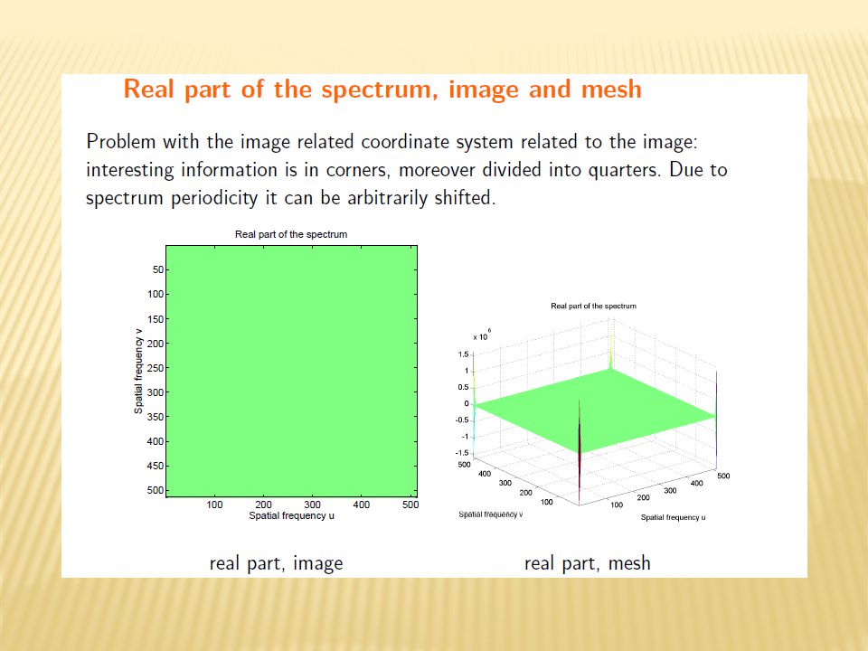
49. Conventional Display for 2-D DFT High frequency area Low frequency area F(u,v) has low frequency areas at corners of the image while high frequency areas are at the center of the image which is inconvenient to interpret.

50. 2-D FFT Shift : Better Display of 2-D DFT 2D FFTSHIFT 2-D FFT Shift is a MATLAB function: Shift the zero frequency of F(u,v) to the center of an image. High frequency areaLow frequency area

51. Original display of 2D DFT 0N2N-N 0 M 2M -M Display of 2D DFT After FFT Shift 2-D FFT Shift : How it works

52. Example of 2-D DFT Original image 2D DFT 2D FFT Shift

53. Example of 2-D DFT Original image 2D DFT 2D FFT Shift

54. Spectrum shift Original image Log enhanced transform Shifted log enhanced transform

57. Computing DFT – Use the two-dimensional FFT command E=fft2(A) – Puts center of the beam in the corners – Use the fftshift command to put it into the center A=imread(‘slit’, ‘gif’) fft2( A ) fftshift( fft2( A ) )

58. DFT Properties: Rotation Rotating f(x,y) by θ rotates F(u,v) by θ

59. DFT DFT Properties: Rotation

60. The Property of Two-Dimensional DFT Linear Combination The Property of Two-Dimensional DFT Linear Combination DFT A B 0.25 * A + 0.75 * B

61. Two-Dimensional DFT with Different Functions Sine wave Rectangle Its DFT

62. Two-Dimensional DFT with Different Functions 2D Gaussian function Impulses Its DFT

63. Two-Dimensional DFT with Different Functions 2D Gaussian function Impulses Its DFT

65. Relation Between Spatial and Frequency Resolutions where  x = spatial resolution in x direction  y = spatial resolution in y direction  u = frequency resolution in x direction  v = frequency resolution in y direction N,M = image width and height  x and  y are pixel width and height. )

66. How to Perform 2-D DFT by Using 1-D DFT f(x,y)f(x,y) 1-D DFT by row F(u,y)F(u,y) 1-D DFT by column F(u,v)F(u,v)

67. How to Perform 2-D DFT by Using 1-D DFT f(x,y)f(x,y) 1-D DFT by row F(x,v)F(x,v) 1-D DFT by column F(u,v)F(u,v) Alternative method

68. Filtering in the Frequency Domain with FFT shift f(x,y)f(x,y) 2D FFT FFT shift F(u,v)F(u,v) 2D IFFTX H(u,v) (User defined) G(u,v)G(u,v) g(x,y)g(x,y) In this case, F(u,v) and H(u,v) must have the same size and have the zero frequency at the center.

77. Smoothing filters: Gaussian The weights are samples of the Gaussian function mask size: σ = 1.4

78. Smoothing filters: Gaussian As σ increases, more samples must be obtained to represent the Gaussian function accurately. Therefore, σ controls the amount of smoothing σ = 3

79. Smoothing filters: Gaussian

84. Fourier Low Pass Filtering

85. Gaussian Low Pass Filter

86. Low pass filtering

96. Fourier High Pass Filtering

97. Linear filtering and convolution DFT IDFT

98. High pass filtering

101. Example of noise reduction using DFT

102. Questions? Discussion? Suggestions ?

103. 102