1. DREAM PLAN IDEA IMPLEMENTATION 1

2. 2

3. 3 Introduction to Image Processing Dr. Kourosh Kiani Email: kkiani2004@yahoo.comkkiani2004@yahoo.com Email: Kourosh.kiani@aut.ac.irKourosh.kiani@aut.ac.ir Email: Kourosh.kiani@semnan.ac.irKourosh.kiani@semnan.ac.ir Web: www.kouroshkiani.comwww.kouroshkiani.com Present to: Amirkabir University of Technology (Tehran Polytechnic) & Semnan University

4. Lecture 03 4

5. POINT OPERATIONS

6. Point Operations Overview Point operations are zero-memory operations where a given gray level x  [0,L] is mapped to another gray level y  [0,L] according to a transformation L L x y L=255: for grayscale images

7. POINT OPERATIONS  A point operation can be defined as a mapping function: where v stands for gray values.  M(v) takes any value v in the source image into v new in the destination image.  Simplest case - Linear Mapping: M(v) v p q p’p’ q’q’

8. L L x y No influence on visual quality at all

9. Digital Negative L x 0 L

10. THE NEGATIVE MAPPING v M(v) 255

11. THE NEGATIVE MAPPING

12. POINT OPERATIONS AND THE HISTOGRAM  Given a point operation:  M(v a ) takes any value v a in image A and maps it into v b in image B.  Requirement: the mapping M is a non descending function (M -1 exists).  In this case, the area under H a between 0 and v a is equal to the area under H b between 0 and v b

13. v v HaHa HbHb M(v) v The area under H a between 0 and v a is equal to the area under H b between 0 and v b =M(v a )

14.  Q: Is it possible to obtain H b directly from H a and M(v)?  A: Since M(v) is monotonic, C a (v a )=C b (v b ) therefore: v v CaCa CbCb M(v) v

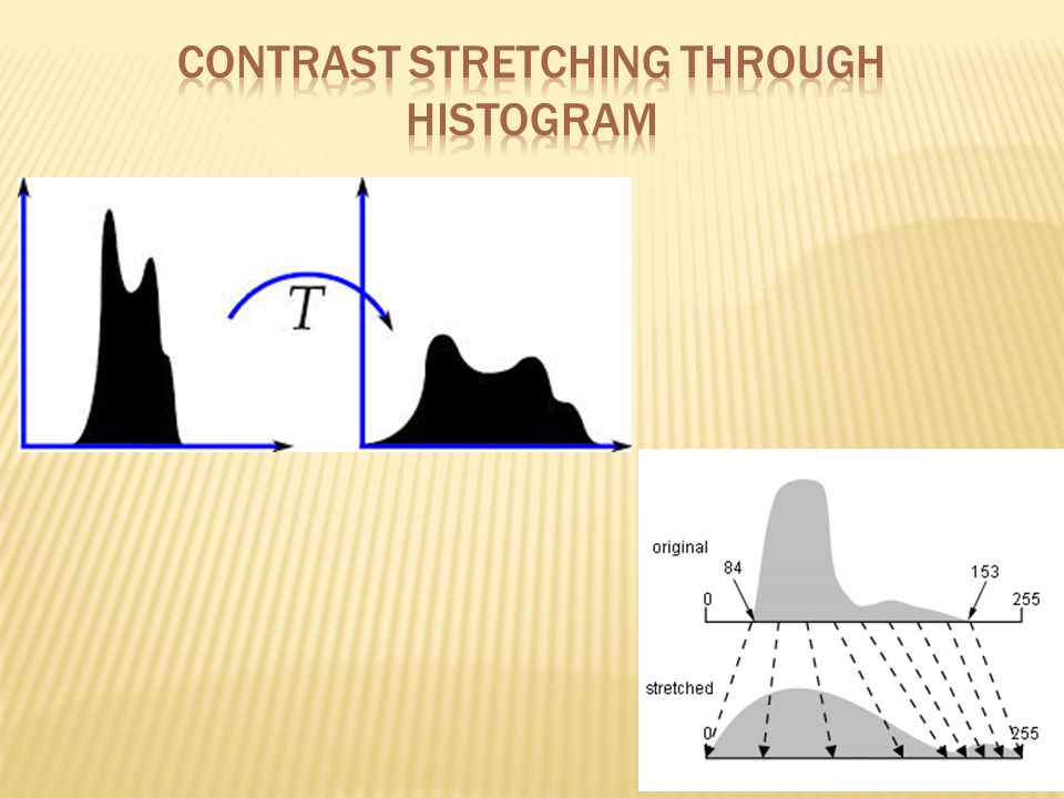
15. Contrast Stretching L x 0 ab yaya ybyb

16. Clipping L x 0 ab

17. Range Compression c=100 L x 0

18. Thresholding transformations are particularly useful for segmentation in which we want to isolate an object of interest from a background s = 1.0 0.0 r <= threshold r > threshold Images taken from Gonzalez & Woods, Digital Image Processing (2002)

19. Original Image x y Image f (x, y) Enhanced Image x y Image f (x, y) s = 0.0 r <= threshold 1.0 r > threshold

20. If r max and r min are the maximum and minimum gray level of the input image and L is the total gray levels of output image The transformation function for contrast stretching will be

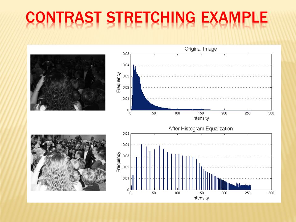
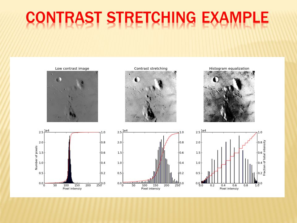
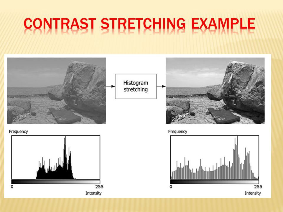
22. One can take an image with a narrow contrast range and expand it to cover the entire range of black to white in a process known as contrast stretching.

27. There are many different kinds of grey level transformations Three of the most common are shown here  Linear  Negative/Identity  Logarithmic  Log/Inverse log  Power law  n th power/n th root

28. The general form of the log transformation is s = c * log(1 + r) The log transformation maps a narrow range of low input grey level values into a wider range of output values The inverse log transformation performs the opposite transformation

29. Log functions are particularly useful when the input grey level values may have an extremely large range of values In the following example the Fourier transform of an image is put through a log transform to reveal more detail s = log(1 + r)

30. Original Image x y Image f (x, y) Enhanced Image x y Image f (x, y) s = log(1 + r) We usually set c to 1 Grey levels must be in the range [0.0, 1.0]

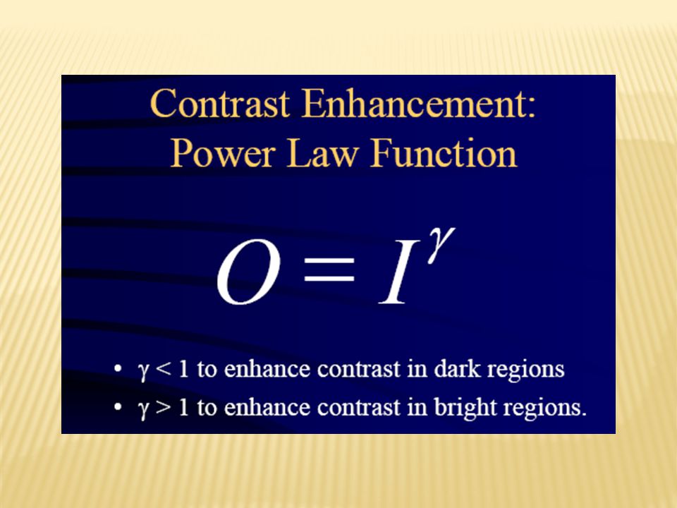
31. Power law transformations have the following form s = c * r γ Map a narrow range of dark input values into a wider range of output values or vice versa Varying γ gives a whole family of curves

32. We usually set c to 1 Grey levels must be in the range [0.0, 1.0] Original Image x y Image f (x, y) Enhanced Image x y Image f (x, y) s = r γ

35. γ = 0.6

36. γ = 0.4

37. γ = 0.3

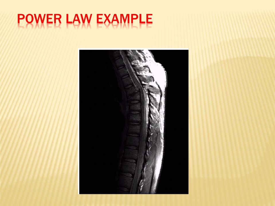
38. The images to the right show a MR image of a fractured human spine Different curves highlight different detail s = r 0.6 s = r 0.4 s = r 0.3

40. γ = 5.0

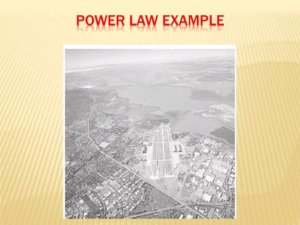
41. An aerial photo of a runway is shown This time power law transforms are used to darken the image Different curves highlight different detail s = r 3.0 s = r 4.0 s = r 5.0

42. Many of you might be familiar with gamma correction of computer monitors Problem is that display devices do not respond linearly to different intensities Can be corrected using a log transform

43.  New Image pixel = (Original Image pixel ) - γ New Image pixel = (Original Image pixel )^-1.5 Original imageNew Image Gamma correction= 1.5

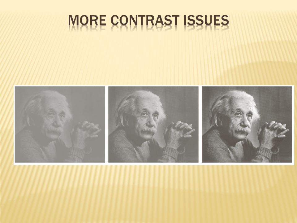
44.  Here is an example at different gammas. L 0, gamma= 1 L 0 2.2, gamma = 1/(2.2) L 0 1/2.2, gamma = 2.2 This is the best gamma

46. Rather than using a well defined mathematical function we can use arbitrary user-defined transforms The images below show a contrast stretching linear transform to add contrast to a poor quality image

47. Highlights a specific range of grey levels  Similar to thresholding  Other levels can be suppressed or maintained  Useful for highlighting features in an image

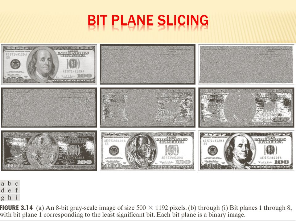
48. Often by isolating particular bits of the pixel values in an image we can highlight interesting aspects of that image  Higher-order bits usually contain most of the significant visual information  Lower-order bits contain subtle details

49. [ 10000000 ] [ 01000000 ] [ 00100000 ] [ 00001000 ] [ 00000100 ] [ 00000001 ] [ 00010000 ] [ 00000010 ]

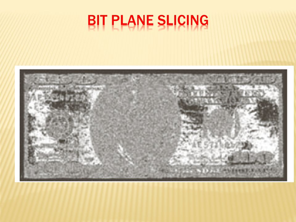
60. Reconstructed image using only bit planes 8 and 7 Reconstructed image using only bit planes 8, 7 and 6 Reconstructed image using only bit planes 7, 6 and 5

61.  Simple gray level transformations  Image negatives  Log transformations  Power-law transformations  Contrast stretching  Gray-level slicing  Bit-plane slicing  Histogram processing  Histogram equalization  Histogram matching (specification)  Arithmetic/logic operations  Image averaging

62. Questions? Discussion? Suggestions ?

63. 63