Download presentation
Presentation is loading. Please wait.

1
Digital Image Processing Chapter 4: Image Enhancement in the Frequency Domain

2
Background The French mathematiian Jean Baptiste Joseph Fourier Born in 1768 Published Fourier series in 1822 Fourier ’ s ideas were met with skepticism Fourier series Any periodical function can be expressed as the sum of sines and/or cosines of different frequencies, each multiplied by a different coefficient

4
Fourier transform Functions can be expressed as the integral of sines and/or cosines multiplied by a weighting function Functions expressed in either a Fourier series or transform can be reconstructed completely via an inverse process with no loss of information

5
Applications Heat diffusion Fast Fourier transform (FFT) developed in the late 1950s
 developed in the late 1950s")
6
Introduction to the Fourier Transform and the Frequency Domain The one-dimensional Fourier transform and its inverse Fourier transform Inverse Fourier transform

7
Two variables Fourier transform Inverse Fourier transform

8
Discrete Fourier transform (DFT) Original variable Transformed variable
 Original variable Transformed variable")
10
DFT The discrete Fourier transform and its inverse always exist f(x) is finite in the book
 is finite in the book")
11
Sines and cosines

12
Time domain Time components Frequency domain Frequency components

13
Fourier transform and a glass prism Prism Separates light into various color components, each depending on its wavelength (or frequency) content Fourier transform Separates a function into various components, also based on frequency content Mathematical prism
 content Fourier transform Separates a function into various components, also based on frequency content Mathematical prism")
14
Polar coordinates Real part Imaginary part

15
Magnitude or spectrum Phase angle or phase spectrum Power spectrum or spectral density

17
Samples

18
Some references http://local.wasp.uwa.edu.au/~pbourk e/other/dft/ http://local.wasp.uwa.edu.au/~pbourk e/other/dft/ http://homepages.inf.ed.ac.uk/rbf/HIP R2/fourier.htm http://homepages.inf.ed.ac.uk/rbf/HIP R2/fourier.htm

19
Examples test_fft.c test_fft.c fft.h fft.h fft.c fft.c Fig4.03(a).bmp Fig4.03(a).bmp test_fig2.bmp test_fig2.bmp
.bmp Fig4.03(a).bmp test_fig2.bmp test_fig2.bmp")
20
The two-dimensional DFT and its inverse

21
Spatial, or image variables: x, y Transform, or frequency variables: u, v

22
Magnitude or spectrum Phase angle or phase spectrum Power spectrum or spectral density

23
Centering Average gray level F(0,0) is called the dc component of the spectrum
 is called the dc component of the spectrum")
24
Conjugate symmetric If f(x,y) is real Relationships between samples in the spatial and frequency domains
 is real Relationships between samples in the spatial and frequency domains")
25
The separation of spectrum zeros in the u-direction is exactly twice the separation of zeros in the v direction

26
Filtering in the frequency domain

27
Strong edges that run approximately at +45 degree, and -45 degree The inclination off horizontal of the long white element is related to a vertical component that is off-axis slightly to the left The zeros in the vertical frequency component correspond to the narrow vertical span of the oxide protrusions

28
Basics of filtering in the frequency domain 1. Multiply the input image by to center the transform 2. Compute F(u,v) 3. Multiply F(u,v) by a filter function H(u,v) 4. Compute the inverse DFT 5. Obtain the real part 6. Multiply the result by
 3. Multiply F(u,v) by a filter function H(u,v) 4. Compute the inverse DFT 5. Obtain the real part 6. Multiply the result by.")
29
Fourier transform of the output image zero-phase-shift filter Real H(u,v)
")
30
Inverse Fourier transform of G(u,v) The imaginary components of the inverse transform should all be zero When the input image and the filter function are real
 The imaginary components of the inverse transform should all be zero When the input image and the filter function are real")
32
Set F(0,0) to be zero, a notch filter
 to be zero, a notch filter")
34
Lowpass filter Pass low frequencies, attenuate high frequencies Blurring Highpass filter Pass high frequencies, attenuate low frequencies Edges, noise

36
Convolution theorem

37
Impulse function of strength A

41
Gaussian filter

43
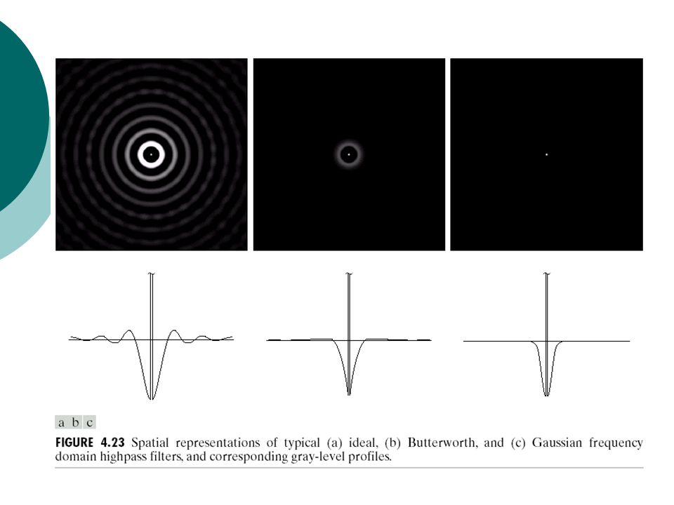
Highpass filter

44
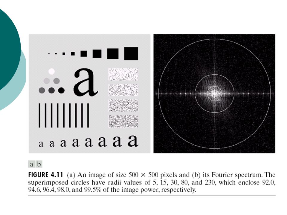
Smoothing Frequency-Domain Filterers Ideal lowpass filters

46
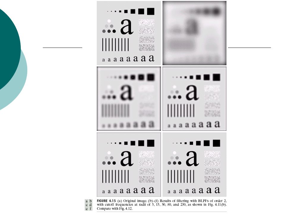
Cutoff frequency Total image power Portion of the total power

49
Blurring and ringing properties Filter Convolution : Spatial filter was multiplied by Then the inverse DFT The real part of the inverse DFT was multiplied by

51
The filter A dominant component at the origin Concentric, circular components about the center component --- ringing The radius of the center component and the number of circles per unit distance from the origin are inversely proportional to the value of the cutoff frequency of the ideal filter.

52
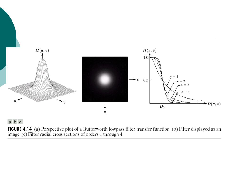
Butterworth lowpass filters when

55
Butterworth lowpass filters Order 1: No ringing Order 2: Imperceptible ringing Higher order: Ringing becomes a significant factor

57
Gaussain lowpass filters When No ringing

60
Additional examples of lowpass filters Machine perception Printing and publishing Satellite and aerial images

64
Sharpening Frequency Domain Filters Highpass filter Spatial filter: was multiplied by Then the inverse DFT The real part of the inverse DFT was multiplied by

67
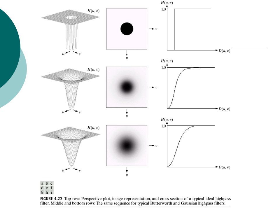
Ideal highpass filters

69
Butterworth highpass filters

71
Gaussian highpass filters

73
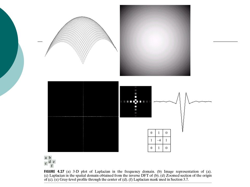
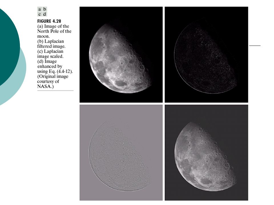
The Laplacian in the frequency domain

74
After centering

75
Inverse Fourier transform Fourier-transform pair

77
Subtracting the Laplacian from the original image

79
Unsharp masking, high-boost filtering, and high-frequency emphasis filtering Highpass filtering High-boost filtering

80
Frequency domain

82
High-frequency emphasis where and

84
Homomorphic Filtering Illumination and reflectance components Derivations

85
Or

86
Frequency domain Spatial domain

88
Decrease the contribution made by the low frequencies (illumination) Amplify the contribution made by high frequencies (reflectance) Simultaneous dynamic range compression and contrast enhancement
 Amplify the contribution made by high frequencies (reflectance) Simultaneous dynamic range compression and contrast enhancement")
91
Implementation Translation When and

93
Distributivity and scaling

94
Rotation Polar coordinates Rotating by an angle rotates by the same angle

95
Periodicity and conjugate symmetry Periodicity property

96
Conjugate symmetry Symmetry of the spectrum

98
Separability

99
where We can compute the 2-D transform by first computing a 1-D transform along each row of the input image, and then computing a 1-D transform along each column of this intermediate result

101
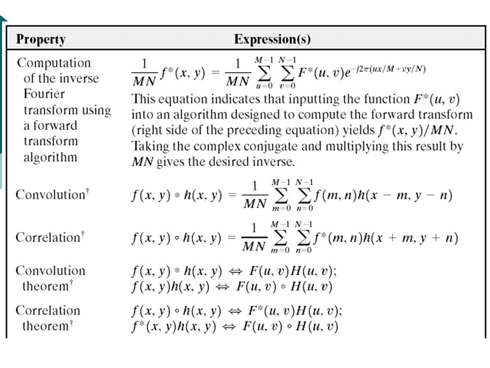
Computing the inverse Fourier transform using a forward transform algorithm

102
Calculate

103
Inputting into an algorithm designed to compute the forward transform gives the quantity

104
2-D

105
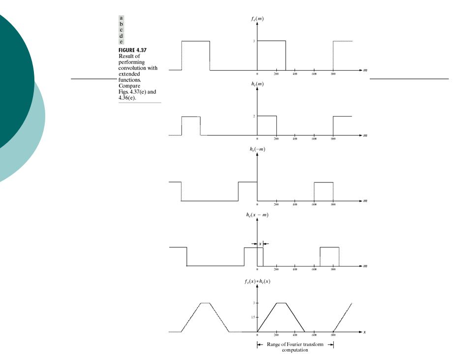
More on periodicity: the need for padding Convolution: Flip one of the functions and slide it pass the other

Similar presentations


>")
>")


>")


>")


![Reminder Fourier Basis: t [0,1] nZnZ Fourier Series: Fourier Coefficient:](/16/4936498/big_thumb.jpg "Reminder Fourier Basis: t [0,1] nZnZ Fourier Series: Fourier Coefficient:>")


