Download presentation
Presentation is loading. Please wait.

1
Computational Photography Prof. Feng Liu Spring 2015 http://www.cs.pdx.edu/~fliu/courses/cs510/ 04/06/2015

2
Last Time Digital Camera History of Camera Controlling Camera Photography Concepts

3
Today Filters and its applications naïve denoising Gaussian blur better denoising edge-preserving filter noisy image Slide credit: Sylvain Paris and Frédo Durand

4
The raster image (pixel matrix) Slide credit: D. Hoiem
 Slide credit: D. Hoiem")
5
The raster image (pixel matrix) 0.920.930.940.970.620.370.850.970.930.920.99 0.950.890.820.890.560.310.750.920.810.950.91 0.890.720.510.550.510.420.570.410.490.910.92 0.960.950.880.940.560.460.910.870.900.970.95 0.710.81 0.870.570.370.800.880.890.790.85 0.490.620.600.580.500.600.580.500.610.450.33 0.860.840.740.580.510.390.730.920.910.490.74 0.960.670.540.850.480.370.880.900.940.820.93 0.690.490.560.660.430.420.770.730.710.900.99 0.790.730.900.670.330.610.690.790.730.930.97 0.910.940.890.490.410.78 0.770.890.990.93 Slide credit: D. Hoiem

6
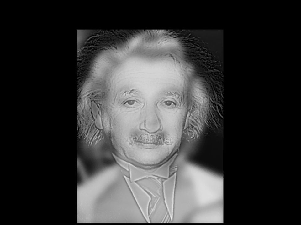
Perception of Intensity Slide credit: T. Adelson

7
Perception of Intensity

8
Color Image R G B Slide credit: D. Hoiem

9
Image filtering: compute function of local neighborhood at each pixel position One type of “Local operator,” “Neighborhood operator,” “Window operator” Useful for: Enhancing images Noise reduction, smooth, resize, increase contrast, etc. Extracting information from images Texture, edges, distinctive points, etc. Detecting patterns Template matching, e.g., eye template Source: D. Hoiem Image Filtering Slide credit: C. Dyer

10
Source: http://lullaby.homepage.dk/diy-camera/bokeh.html Bokeh: Blur in out-of-focus regions of image Camera shake * = Source: Fergus, et al. “Removing Camera Shake from a Single Photograph”, SIGGRAPH 2006 Blurring in the Real World Slide credit: C. Dyer

11
Image Correlation Filtering Select a filter g g is called a filter, mask, kernel, or template Center filter g at each pixel in image f Multiply weights by corresponding pixels Set resulting value in output image h Linear filtering is sum of dot product at each pixel position Filtering operation called cross-correlation, and denoted h = f g Slide credit: C. Dyer

12
111 111 111 Example: Box Filter Slide credit: David Lowe

13
0000000000 0000000000 00090 00 000 00 000 00 000 0 00 000 00 0000000000 00 0000000 0000000000 0 0000000000 0000000000 000 00 000 00 000 00 000 0 00 000 00 0000000000 00 0000000 0000000000 Credit: S. Seitz Image Filtering 111 111 111

14
0000000000 0000000000 00090 00 000 00 000 00 000 0 00 000 00 0000000000 00 0000000 0000000000 010 0000000000 0000000000 00090 00 000 00 000 00 000 0 00 000 00 0000000000 00 0000000 0000000000 Image Filtering 111 111 111 Credit: S. Seitz

15
0000000000 0000000000 00090 00 000 00 000 00 000 0 00 000 00 0000000000 00 0000000 0000000000 01020 0000000000 0000000000 00090 00 000 00 000 00 000 0 00 000 00 0000000000 00 0000000 0000000000 Image Filtering 111 111 111 Credit: S. Seitz

16
0000000000 0000000000 00090 00 000 00 000 00 000 0 00 000 00 0000000000 00 0000000 0000000000 0102030 0000000000 0000000000 00090 00 000 00 000 00 000 0 00 000 00 0000000000 00 0000000 0000000000 Image Filtering 111 111 111 Credit: S. Seitz

17
0102030 0000000000 0000000000 00090 00 000 00 000 00 000 0 00 000 00 0000000000 00 0000000 0000000000 Image Filtering 111 111 111 Credit: S. Seitz

18
0102030 0000000000 0000000000 00090 00 000 00 000 00 000 0 00 000 00 0000000000 00 0000000 0000000000 Image Filtering 111 111 111 ? Credit: S. Seitz

19
0102030 50 0000000000 0000000000 00090 00 000 00 000 00 000 0 00 000 00 0000000000 00 0000000 0000000000 Image Filtering 111 111 111 ? Credit: S. Seitz

20
0000000000 0000000000 00090 00 000 00 000 00 000 0 00 000 00 0000000000 00 0000000 0000000000 0102030 2010 0204060 4020 0306090 6030 0 5080 906030 0 5080 906030 0203050 604020 102030 2010 00000 Image Filtering 111 111 111 Credit: S. Seitz

21
What does it do? Replaces each pixel with an average of its neighborhood Achieves smoothing effect (i.e., removes sharp features) Weaknesses: Blocky results Axis-aligned streaks 111 111 111 Slide credit: David Lowe Box Filter
 Weaknesses: Blocky results Axis-aligned streaks Slide credit: David Lowe Box Filter.")
22
Smoothing with Box Filter Slide credit: C. Dyer

23
Properties of Smoothing Filters Smoothing Values all positive Sum to 1 constant regions same as input Amount of smoothing proportional to mask size Removes “high-frequency” components “low-pass” filter Slide credit: C. Dyer

24
Weight contributions of neighboring pixels by nearness Constant factor at front makes volume sum to 1 Convolve each row of image with 1D kernel to produce new image; then convolve each column of new image with same 1D kernel to yield output image 0.003 0.013 0.022 0.013 0.003 0.013 0.059 0.097 0.059 0.013 0.022 0.097 0.159 0.097 0.022 0.013 0.059 0.097 0.059 0.013 0.003 0.013 0.022 0.013 0.003 5 x 5, = 1 Slide credit: Christopher Rasmussen Gaussian Filtering

25
Smoothing with a box actually doesn’t compare at all well with a defocused lens Most obvious difference is that a single point of light viewed in a defocused lens looks like a fuzzy blob; but the averaging process would give a little square Gaussian is isotropic (i.e., rotationally symmetric) A Gaussian gives a good model of a fuzzy blob It closely models many physical processes (the sum of many small effects) Slide by D.A. Forsyth Smoothing with a Gaussian

26
What does Blurring take away? original Slide credit: C. Dyer

27
What does Blurring take away? smoothed (5x5 Gaussian) Slide credit: C. Dyer
 Slide credit: C. Dyer")
28
Smoothing with Gaussian Filter

29
Smoothing with Box Filter

30
input Slide by S. Paris

31
box average Slide by S. Paris

32
Gaussian blur Slide by S. Paris

33
What parameters matter here? Standard deviation, , of Gaussian: determines extent of smoothing σ = 2 with 30 x 30 kernel σ = 5 with 30 x 30 kernel Source: D. Hoiem Gaussian Filters

34
Slide credit: C. Dyer

35
for sigma=1:3:10 h = fspecial('gaussian‘, hsize, sigma); out = imfilter(im, h); imshow(out); pause; end … Parameter σ is the “scale” / “width” / “spread” of the Gaussian kernel, and controls the amount of smoothing Smoothing with a Gaussian Slide credit: C. Dyer

36
Gaussian filters = 30 pixels= 1 pixel = 5 pixels = 10 pixels Slide credit: C. Dyer

37
What parameters matter here? Size of kernel or mask σ = 5 with 10 x 10 kernel σ = 5 with 30 x 30 kernel Gaussian Filters Slide credit: C. Dyer

38
Gaussian function has infinite “support” but need a finite-size kernel Values at edges should be near 0 98.8% of area under Gaussian in mask of size 5σ x 5σ In practice, use mask of size 2k+1 x 2k+1 where k 3 Normalize output by dividing by sum of all weights How big should the filter be? Slide credit: C. Dyer

39
Original 111 111 111 000 020 000 - ? (Note that filter sums to 1) Source: D. Lowe Sharpening Filters

40
Original 111 111 111 000 020 000 - Sharpening filter - Sharpen an out of focus image by subtracting a multiple of a blurred version Source: D. Lowe Sharpening Filters

41
Source: D. Lowe Sharpening

42
h = f + k(f * g) where k is a small positive constant and g = Called unsharp masking in photography 010 1-41 010 called a Laplacian mask Sharpening by Unsharp Masking
 where k is a small positive constant and g = Called unsharp masking in photography called a Laplacian mask Sharpening by Unsharp Masking")
43
Sharpening using Unsharp Mask Filter OriginalFiltered result Slide credit: C. Dyer

44
01 -202 01 Vertical Edge (absolute value) Sobel Application: Edge Detection Slide credit: C. Dyer
 Sobel Application: Edge Detection Slide credit: C. Dyer")
45
-2 000 121 Horizontal Edge (absolute value) Sobel Application: Edge Detection Slide credit: C. Dyer
 Sobel Application: Edge Detection Slide credit: C. Dyer")
46
Application: Hybrid Images Gaussian Filter Laplacian Filter A. Oliva, A. Torralba, P.G. Schyns, Hybrid Images, SIGGRAPH 2006 Gaussian unit impulse Laplacian of Gaussian I1I1 I2I2 G1G1 (1-G 2 ) I1 G1I1 G1
 I1 G1I1 G1.")
48
Application: XDoG Filters Gaussian filtering results Winnemoller, H., XDoG: advanced image stylization with eXtended Difference-of-Gaussians NPAR 2011 Input XDoG Input XDoG

49
Application: Painterly Filters Many methods have been proposed to make a photo look like a painting Today we look at one: Painterly-Rendering with Brushes of Multiple Sizes Basic ideas: Build painting one layer at a time, from biggest to smallest brushes At each layer, add detail missing from previous layer A. Hertzmann, Painterly rendering with curved brush strokes of multiple sizes, SIGGRAPH 1998. Slide credit: S. Chenney

50
Algorithm 1 function paint(sourceImage,R 1... R n ) // take source and several brush sizes { canvas := a new constant color image // paint the canvas with decreasing sized brushes for each brush radius R i, from largest to smallest do { // Apply Gaussian smoothing with a filter of size const * radius // Brush is intended to catch features at this scale referenceImage = sourceImage * G(fs R i ) // Paint a layer paintLayer(canvas, referenceImage, Ri) } return canvas } Slide credit: S. Chenney
 // take source and several brush sizes { canvas := a new constant color image // paint the canvas with decreasing sized brushes for each brush radius R i, from largest to smallest do { // Apply Gaussian smoothing with a filter of size const * radius // Brush is intended to catch features at this scale referenceImage = sourceImage * G(fs R i ) // Paint a layer paintLayer(canvas, referenceImage, Ri) } return canvas } Slide credit: S. Chenney.")
51
Algorithm 2 procedure paintLayer(canvas,referenceImage, R) // Add a layer of strokes { S := a new set of strokes, initially empty D := difference(canvas,referenceImage) // euclidean distance at every pixel for x=0 to imageWidth stepsize grid do // step in size that depends on brush radius for y=0 to imageHeight stepsize grid do { // sum the error near (x,y) M := the region (x-grid/2..x+grid/2, y-grid/2..y+grid/2) areaError := sum(D i,j for i,j in M) / grid 2 if (areaError > T) then { // find the largest error point (x1,y1) := max D i,j in M s :=makeStroke(R,x1,y1,referenceImage) add s to S } paint all strokes in S on the canvas, in random order } Slide credit: S. Chenney

52
Results OriginalBiggest brush Medium brush addedFinest brush added Slide credit: S. Chenney

53
Next Time More Filters De-noise

Similar presentations

>")


 in an image Intuitively, most semantic and shape information from the image can be encoded.>")


 Images by Pawan SinhaPawan Sinha formal terminology.>")


