Download presentation
Presentation is loading. Please wait.

1
CS 4487/9587 Algorithms for Image Analysis
Image Processing Basics Lecture 3 Lena Gorelick, substituting for Yuri Boykov Acknowledgements: slides from Steven Seitz, Aleosha Efros, David Forsyth, and Gonzalez & Woods

2
CS 4487/9587 Algorithms for Image Analysis Image Processing Basics
Domain Transformation Resize, Rotate etc. Range Transformation Point Processing gamma correction window-center correction histogram equalization Pixel location Pixel Intensity Window = 800 Center = 1160

3
CS 4487/9587 Algorithms for Image Analysis Image Processing Basics
Domain Transformation Resize, Rotate etc. Range Transformation Point Processing gamma correction window-center correction histogram equalization Neighborhood Processing (Filtering)
")
4
Neighborhood Processing (or filtering)
What is wrong with this image? How can we remove noise? Look spatially around each pixel - neighborhood Can we use Point Processing? Courtesy of Carlo Tomasi Courtesy of Neel Joshi Readings: Forsyth & Ponce, chapters

5
Neighborhood Processing (or filtering)
Lets reshuffle all pixels within the image Point Processing will have the same effect Gets intensity of a single pixel as an input Unaware of spatial information Neighborhood Processing Takes “spatial information” into account Images contain “spatial information” Has Spatial Information Looks noisy Readings: Forsyth & Ponce, chapters

6
Neighborhood Processing (filtering) Linear image transforms
Assume 1D function

7
Neighborhood Processing (filtering) Linear image transforms
Assume 1D function

8
Neighborhood Processing (filtering) Linear shift-invariant filters
matrix M A commonly used pattern Represented by a kernel (or a mask) For 2k+1 size kernel Shift - Invariant The same in each row (i - 1) i (i + 1)
 For 2k+1 size kernel. Shift - Invariant. The same in each row. (i - 1) i. (i + 1)")
9
Neighborhood Processing (filtering) 2D linear transforms
Assume 2D function Concatenate the columns using a “raster-scan” order

10
Neighborhood Processing (filtering) 2D filtering
A 2D function Can be filtered by a 2D filter (kernel) To get a new image This is called a cross-correlation operation Or a sliding dot-product
 To get a new image. This is called a cross-correlation operation Or a sliding dot-product.")
11
Neighborhood Processing (filtering) 2D filtering
Cross-correlation in which the filter is flipped horizontally and vertically is called convolution

12
Neighborhood Processing (filtering) Convolution vs. Cross-Correlation
If the kernel is symmetric convolution = cross-correlation

13
Neighborhood Processing 2D filtering Noise
Types of noise: Salt and pepper noise Impulse noise Gaussian noise Due to transmission errors dead CCD pixels specks on lens can be specific to a sensor Salt and pepper and impulse noise can be due to transmission errors (e.g., from deep space probe), dead CCD pixels, specks on lens We’re going to focus on Gaussian noise first. If you had a sensor that was a little noisy and measuring the same thing over and over, how would you reduce the noise?
, dead CCD pixels, specks on lens. We’re going to focus on Gaussian noise first. If you had a sensor that was a little noisy and measuring the same thing over and over, how would you reduce the noise")
14
Neighborhood Processing Practical Noise Reduction
How can we remove noise? Replace each pixel with the average of a kxk window around it 100 130 110 120 90 80 104

15
Neighborhood Processing (filtering) Mean filtering
90 Replace each pixel with the average of a kxk window around it

16
Neighborhood Processing (filtering) Mean filtering
90 10 20 30 40 60 90 50 80 Replace each pixel with the average of a kxk window around it What happens if we use a larger filter window?

17
Neighborhood Processing (filtering) Effect of mean filters
3x3 5x5 7x7 Salt & Pepper noise Gaussian noise Demo with photoshop Side effect - blur

18
Neighborhood Processing (filtering) Mean kernel
What’s the kernel for a 3x3 mean filter? 90

19
Neighborhood Processing (filtering) Mean kernel
What’s the kernel for a 3x3 mean filter? 90 1/9

20
Neighborhood Processing (filtering) Mean kernel
What’s the kernel for a 3x3 mean filter? Equal weight to all pixels within the neighborhood 90 1 1/9

21
Neighborhood Processing (filtering) Gaussian Filtering
A Gaussian kernel gives less weight to pixels further from the center of the window 90 1 2 4 is a discrete approximation of a Gaussian function:

22
Neighborhood Processing (filtering) Mean vs. Gaussian filtering
Input image Gaussian filtering Mean Filtering Gaussian filter, 20x20, σ = 5 Mean filter, 20x20

23
Neighborhood Processing (filtering) Mean vs. Gaussian filtering
 Mean vs. Gaussian filtering")
24
Neighborhood Processing (filtering) Gaussian Filtering
Low-pass filter Smooth color variation (low frequency) is preserved Sharp edges (high frequency) are removed
 is preserved. Sharp edges (high frequency) are removed.")
25
Neighborhood Processing (filtering) Median filters
A Median Filter operates over a window by selecting the median intensity in the window. Image credit: Wikipedia – page on Median Filter

26
Neighborhood Processing (filtering) Median filters
Is a median filter a kind of convolution? No, median filter is an example of non-linear filtering

27
Salt&Pepper Noise

28
Gaussian noise

29
Neighborhood Processing (filtering) Median filters
What advantage does a median filter have over a mean filter? Better at removing Salt & Pepper noise Disadvantage: Slow Better at salt’n’pepper noise Not convolution: try a region with 1’s and a 2, and then 1’s and a 3

30
Neighborhood Processing (filtering) Derivatives and Convolution
Image Derivatives and Gradients Used for Edge/Corner Detection Computed with Finite Differences Filters Laplacian of Gaussians (LoG) Filter Used for Edge/Blob Detection and Image Enhancement Approximated using Difference of Gaussians
 Filter. Used for Edge/Blob Detection and Image Enhancement. Approximated using Difference of Gaussians.")
31
Reading: Forsyth & Ponce, 8.1-8.2 First Derivative
Recall Sharp changes in gray level of the input image correspond to “peaks or valleys” of the first-derivative of the input signal.

32
Reading: Forsyth & Ponce, 8.1-8.2 First Derivative and convolution
How can we approximate it for a discrete function? Is this operation shift-invariant? Is it linear? ?

33
Reading: Forsyth & Ponce, 8.1-8.2 First Derivative and convolution
Finite Difference x x+h x x-h x x+h/2 x-h/2 Slide credit: Wikipedia

34
Reading: Forsyth & Ponce, 8.1-8.2 First Derivative and convolution
Finite Difference – The order of an error can be derived using Taylor Theorem Slide credit: Wikipedia

35
Reading: Forsyth & Ponce, 8.1-8.2 First Derivative and convolution
Pixel Size Using Finite Central Difference We need a kernel such that 1 -1

36
Neighborhood Processing (filtering) Finite differences – responds to edges
Now the figure on the right is signed; darker is negative, lighter is positive, and mid grey is zero. I always ask 1) which derivative (y or x) is this? 2) Have I got the sign of the kernel right? (i.e. is it d/dx or -d/dx). Dark = negative White = positive Gray = 0
 which derivative (y or x) is this 2) Have I got the sign of the kernel right (i.e. is it d/dx or -d/dx). Dark = negative White = positive Gray = 0")
37
Increasing noise -> (this is zero mean additive gaussian noise)
Neighborhood Processing (filtering) Finite differences - responding to noise Increasing noise -> (this is zero mean additive gaussian noise)
 Finite differences - responding to noise. Increasing noise -> (this is zero mean additive gaussian noise)")
38
Neighborhood Processing (filtering) Finite differences and noise
Finite difference filters respond strongly to noise Noisy pixels look very different from their neighbours The larger the noise the stronger is the response How can we eliminate the response to noise? Most pixels in images look similar to their neighbours (even at an edge) Smooth the image (mean/gaussian filtering)
 Smooth the image (mean/gaussian filtering)")
39
Neighborhood Processing (filtering) Smoothing and Differentiation
Smoothing before differentiation = two convolutions Convolution is associative Important to point out that the derivative of gaussian kernels I’ve illustrated “look like” the effects that they’re trying to identify.

40
Neighborhood Processing (filtering) Smoothing and Differentiation
1 pixel 3 pixels 7 pixels The scale of the smoothing filter affects derivative estimates, and also the semantics of the edges recovered.

41
Sobel kernels Yet another approximation frequently used
Neighborhood Processing (filtering) Sobel kernels Yet another approximation frequently used 1 -1 2 -2 1 2 -1 -2
 Sobel kernels. Yet another approximation frequently used")
42
Neighborhood Processing (filtering) Image Gradients
Recall for a function of two variables The gradient at a point (x,y) Gradient Magnitude Gradient Orientation direction of the “steepest ascend” orthogonal to object boundaries in the image x y small image gradients in low textured areas
 Gradient Magnitude. Gradient Orientation. direction of the steepest ascend orthogonal to object boundaries in the image. x. y. small image. gradients in low. textured areas.")
43
Neighborhood Processing (filtering) Image Gradient for Edge Detection
Typical application where image gradients are used is image edge detection find points with large image gradients Canny edge detector suppresses non-extrema Gradient points

44
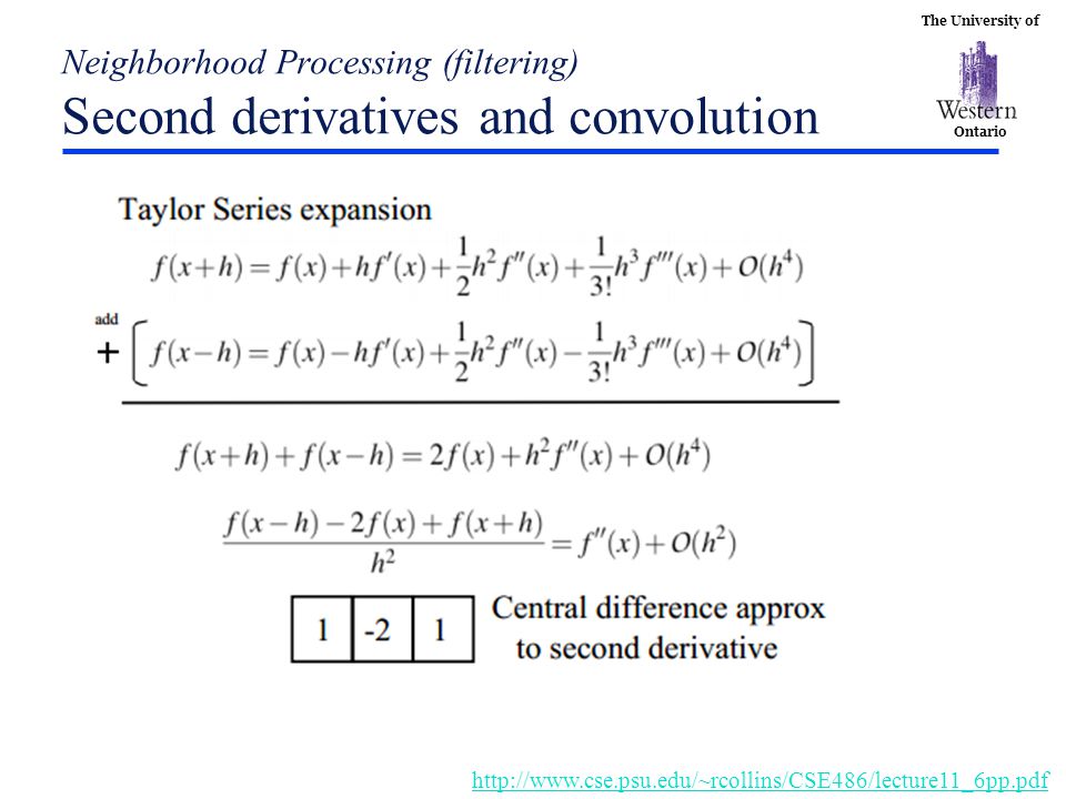
Reading: Forsyth & Ponce, 8.1-8.2 Second derivatives and convolution
Peaks or valleys of the first-derivative of the input signal, correspond to “zero-crossings” of the second-derivative of the input signal.

45
Neighborhood Processing (filtering) Second derivatives and convolution
46
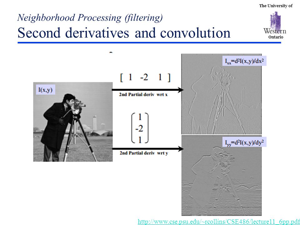
Neighborhood Processing (filtering) Second derivatives and convolution
Better localized edges But more sensitive to noise

47
Neighborhood Processing (filtering) Second derivatives and convolution
48
Neighborhood Processing (filtering) Second Image Derivatives
Laplace operator “divergence of gradient” rotationally invariant second derivative for 2D functions is the rate at which the average value of ƒ over spheres centered atp, deviates from ƒ(p) as the radius of the sphere grows. -1 2 -1 2 -1 4 Finite Difference Second Order Derivative in x Finite Difference Second Order Derivative in y
 as the radius of the sphere grows Finite Difference. Second Order. Derivative in x. Finite Difference. Second Order. Derivative in y.")
49
Neighborhood Processing (filtering) Second Image Derivatives
Laplacian Zero Crossing Used for edge detection (alternative to computing Gradient extrema) image intensity Non-decreasing function slow increase, faster increase, slow increase Positive gradient Positive Magnitude of gradient magnitude of image gradient Laplacian (2nd derivative) of the image
 image. intensity. Non-decreasing function slow increase, faster increase, slow increase. Positive gradient. Positive Magnitude of gradient magnitude of. image gradient. Laplacian. (2nd derivative) of the image.")
50
Neighborhood Processing (filtering) Laplacian Filtering
-Zero on uniform regions -Positive on one side of an edge -Negative on the other side -Zero at some point in between on the edge itself band-pass filter (Suppresses both high and low frequencies)
")
51
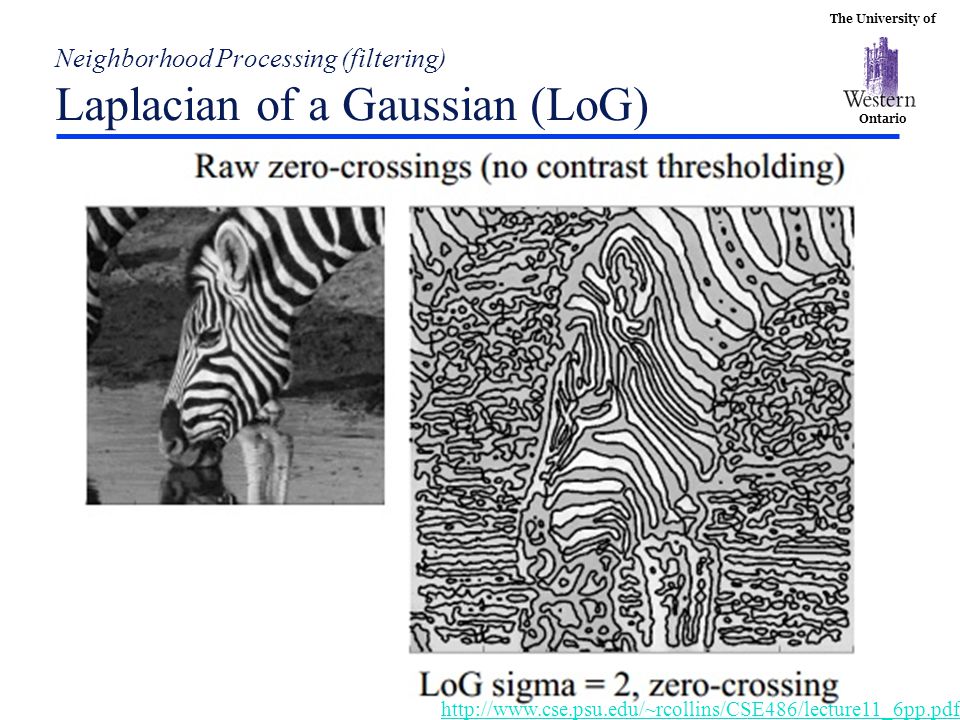
Neighborhood Processing (filtering) Laplacian of a Gaussian (LoG)
Smooth before differentiation (remember associative property of convolution)
")
52
Neighborhood Processing (filtering) Laplacian of a Gaussian (LoG)
Suppresses both high and low frequencies

53
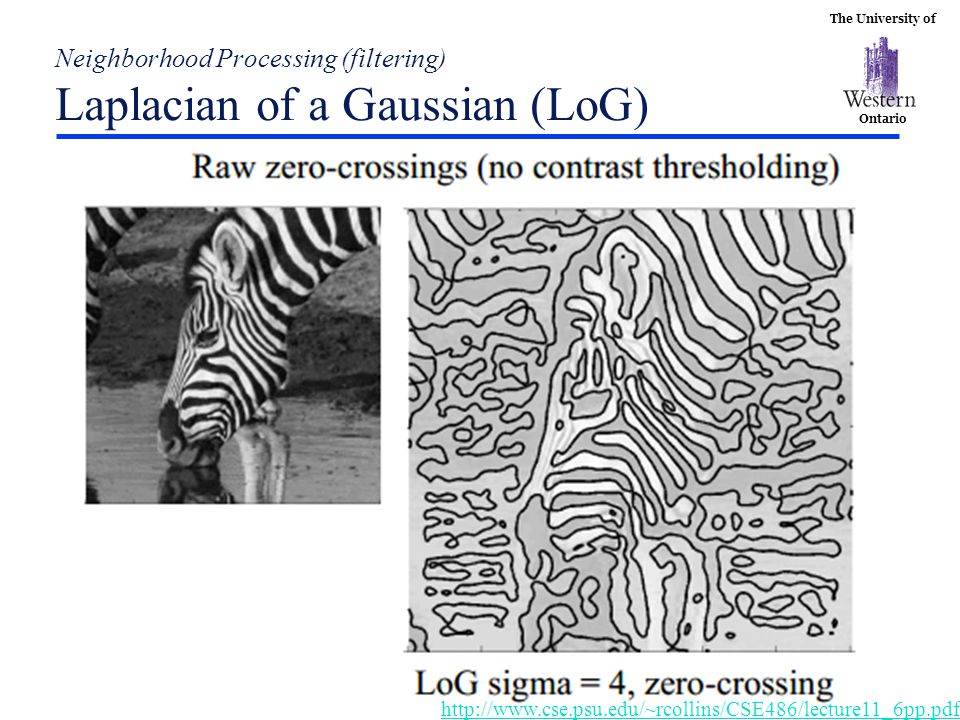
Neighborhood Processing (filtering) Laplacian of a Gaussian (LoG)
54
Neighborhood Processing (filtering) Laplacian of a Gaussian (LoG)
55
Neighborhood Processing (filtering) Laplacian of a Gaussian (LoG)
Can be approximated by a difference of two Gaussians (DoG)
")
56
Neighborhood Processing (filtering) DoG vs. LoG
Separable (product decomposition) more efficient Can explain band-pass filter since Gaussian is a low-pass filter.
 more efficient. Can explain band-pass filter since Gaussian is a low-pass filter.")
57
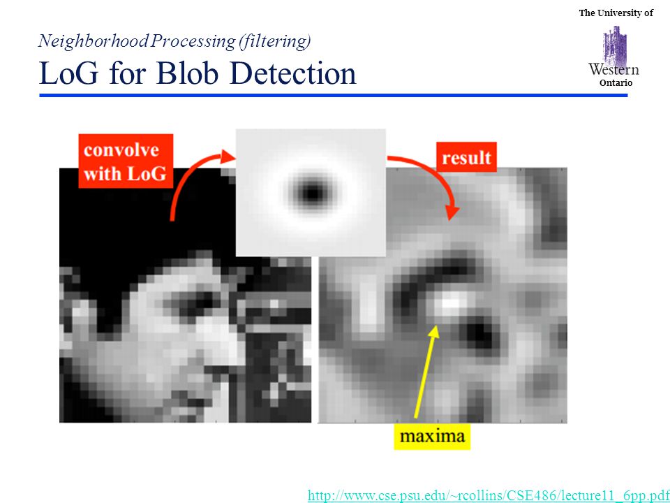
Neighborhood Processing (filtering) LoG for Blob Detection
Cross correlation with a filter can be viewed as comparing a little “picture” of what you want to find against all local regions in the image. Scale of blob (size ; radius in pixels) is determined by the sigma parameter of the LoG filter.
 is determined by the sigma parameter of the LoG filter.")
58
Neighborhood Processing (filtering) LoG for Blob Detection
59
Neighborhood Processing (filtering) Unsharp masking
What does blurring take away? - = unsharp mask +a = ? They are the same for filters that have both horizontal and vertical symmetry. unsharp mask

60
Neighborhood Processing (filtering) Unsharp masking
= ? They are the same for filters that have both horizontal and vertical symmetry. unsharp mask

61
Reading: Forsyth & Ponce ch.7.5 Filters and Templates
Recall: filtering = cross-correlation = dot-product Measures the angle between two vectors: the filter and the image window Measures visual similarity (x,y) Filter Mask Input Image f(x,y) g(x,y) Output Image Correlation
 Filter Mask. Input Image. f(x,y) g(x,y) Output Image. Correlation.")
62
Neighborhood Processing (filtering) Template Matching
Since we divide by the norm Normalized cross-correlation Bring the template and the image to a uniform scale: subtract the mean and divide by the variance

63
Neighborhood Processing (filtering) Template Matching
Normalized cross-correlation Extremely time consuming due to sliding window Slide credit: Matlab manual

64
Neighborhood Processing (filtering) Template Matching
Slide credit: OpenCV manual

Similar presentations


>")


 in an image Intuitively, most semantic and shape information from the image can be encoded.>")


 Images by Pawan SinhaPawan Sinha formal terminology.>")
: A very general and useful class of transforms are the linear transforms of f, defined.>")