1. PowerPoint Presentation Materials to accompany
Genetics: Analysis and Principles
Robert J. Brooker
CHAPTER 5
LINKAGE AND GENETIC MAPPING IN EUKARYOTES
Copyright ©The McGraw-Hill Companies, Inc. Permission required for reproduction or display

2. 5.1 LINKAGE AND CROSSING OVER
In eukaryotic species, each linear chromosome contains a long piece of DNA
A typical chromosome contains many hundred or even a few thousand different genes
The term linkage has two related meanings
1. Two or more genes can be located on the same chromosome
2. Genes that are close together tend to be transmitted as a unit
5-3
Copyright ©The McGraw-Hill Companies, Inc. Permission required for reproduction or display

3. Chromosomes are called linkage groups
They contain a group of genes that are linked together
The number of linkage groups is the number of types of chromosomes of the species
For example, in humans
22 autosomal linkage groups
An X chromosome linkage group
A Y chromosome linkage group
Genes that are far apart on the same chromosome may independently assort from each other
This is due to crossing-over
5-4
Copyright ©The McGraw-Hill Companies, Inc. Permission required for reproduction or display

5. Crossing Over May Produce Recombinant Phenotypes
In diploid eukaryotic species, linkage can be altered during meiosis as a result of crossing over
Crossing over
Occurs during prophase I of meiosis at the bivalent stage
Non-sister chromatids of homologous chromosomes exchange DNA segments
5-5
Copyright ©The McGraw-Hill Companies, Inc. Permission required for reproduction or display

6. Copyright © The McGraw-Hill Companies, Inc
Copyright © The McGraw-Hill Companies, Inc. Permission required for reproduction or display. b b B b B B a a A a A A
Fig. 5.1(TE Art)
Diploid cell after chromosome replication
Diploid cell after chromosome replication
Meiosis
Meiosis B B B B A A A a b b b b a a a A
Possible haploid cells
Possible haploid cells
(a) Without crossing over, linked alleles segregate together.
(b) Crossing over can reassort linked
alleles.

7. These haploid cells contain a combination of alleles NOT found in the original chromosomes
This new combination of alleles is a result of genetic recombination
These are termed parental or non-recombinant cells
These are termed nonparental or recombinant cells
Figure 5.1
5-7

8. Bateson and Punnett Discovered Two Traits That Did Not Assort Independently
In 1905, William Bateson and Reginald Punnett conducted a cross in sweet pea involving two different traits
Flower color and pollen shape
This is a dihybrid cross that is expected to yield a 9:3:3:1 phenotypic ratio in the F2 generation
However, Bateson and Punnett obtained surprising results
5-8
Copyright ©The McGraw-Hill Companies, Inc. Permission required for reproduction or display

9. Figure 5.2
A much greater proportion of the two types found in the parental generation
5-9

10. Morgan Provided Evidence for the Linkage of Several X-linked Genes
The first direct evidence of linkage came from studies of Thomas Hunt Morgan
Morgan investigated several traits that followed an X-linked pattern of inheritance
Figure 5.3 illustrates an experiment involving three traits
Body color
Eye color
Wing length
5-11
Copyright ©The McGraw-Hill Companies, Inc. Permission required for reproduction or display

11. yy ww mm
y+y w+w m+m
F1 generation x
y w m Y
y+ w+ m+ Y
F1 generation contains wild-type females and yellow-bodied, white-eyed, miniature-winged males.

12. Morgan’s explanation: All three genes are located on the X chromosome
P Males
P Females
Morgan observed a much higher proportion of the combinations of traits found in the parental generation
Morgan’s explanation:
All three genes are located on the X chromosome
Therefore, they tend to be transmitted together as a unit
5-13
Copyright ©The McGraw-Hill Companies, Inc. Permission required for reproduction or display

13. Morgan Provided Evidence for the Linkage of Several X-linked Genes
1. Why did the F2 generation have a significant number of nonparental combinations?
2. Why was there a quantitative difference between the various nonparental combinations?
5-14
Copyright ©The McGraw-Hill Companies, Inc. Permission required for reproduction or display

14. White eyes, miniature wings 716 Red eyes, miniature wings 401
Let’s reorganize Morgan’s data by considering the pairs of genes separately
Gray body, red eyes
1,159
Yellow body, white eyes
1,017
Gray body, white eyes 17
Yellow body, red eyes 12
Total
2,205
But this nonparental combination was rare
Red eyes, normal wings
770
White eyes, miniature wings
716
Red eyes, miniature wings
401
White eyes, normal wings
318
Total
2,205
It was fairly common to get this nonparental combination
5-15
Copyright ©The McGraw-Hill Companies, Inc. Permission required for reproduction or display

15. Morgan made three important hypotheses to explain his results
1. The genes for body color, eye color and wing length are all located on the X-chromosome
They tend to be inherited together
2. Due to crossing over, the homologous X chromosomes (in the female) can exchange pieces of chromosomes
This created new combination of alleles
3. The likelihood of crossing over depends on the distance between the two genes
Crossing over is more likely to occur between two genes that are far apart from each other
5-17
Copyright ©The McGraw-Hill Companies, Inc. Permission required for reproduction or display

16. Figure 5-5 Copyright © 2006 Pearson Prentice Hall, Inc.
Figure 5-5 Two examples of a single crossover between two nonsister chromatids and the gametes subsequently produced. In (a) the exchange does not alter the linkage arrangement between the alleles of the two genes, only parental gametes are formed, and the exchange goes undetected. In (b) the exchange separates the alleles, resulting in recombinant gametes, which are detectable.
Figure Copyright © 2006 Pearson Prentice Hall, Inc.

17. Figure 5.4
These parental phenotypes are the most common offspring
These recombinant offspring are not uncommon
5-18
because the genes are far apart

18. 5-19 Figure 5.4 These recombinant offspring are fairly uncommon
because the genes are very close together
These recombinant offspring are very unlikely
1 out of 2,205
5-19

19. Chi Square Analysis
This method is frequently used to determine if the outcome of a dihybrid cross is consistent with linkage or independent assortment
5-20
Copyright ©The McGraw-Hill Companies, Inc. Permission required for reproduction or display

20. Creighton and McClintock Experimentwx
Normal chromosome 9
Parental chromosomes c Wx
Abnormal chromosome 9
Crossing over c wx
Knob
Interchanged piece from
chromosome 8
Nonparental chromosomes
(a) Normal and abnormal chromosome 9 C Wx
C = Colored
c = colorless
Wx = Starchy endosperm
wx = waxy endosperm
(b) Crossing over between normal and
abnormal chromosome 9

21. Figure 5.6
5-30

22. Interpreting the Data Parent A Parent B C wx (nonrecombinant)
C Wx (recombinant)
c wx (recombinant)
c Wx
c wx
By combining these gametes into a Punnett square, the following types of offspring can be produced
5-32
Copyright ©The McGraw-Hill Companies, Inc. Permission required for reproduction or display

23. So let’s start by considering the unambiguous phenotypes
Ambiguous phenotypes that could be produced whether or not recombination occurred in parent A
So let’s start by considering the unambiguous phenotypes
5-33
Copyright ©The McGraw-Hill Companies, Inc. Permission required for reproduction or display

24. The colored, waxy phenotype (Cc wxwx) can occur only if
Recombination did not occur in parent A
AND
Parent A passed the knobbed, translocated chromosome to its offspring
This was the case, as shown in the data table below
5-34
Copyright ©The McGraw-Hill Companies, Inc. Permission required for reproduction or display

25. The colorless, waxy phenotype (cc wxwx) can occur only if
Recombination did occur in parent A
AND
Parent A passed a chromosome 9 that had a translocation but was knobless
This was the case, as shown in the data table below
5-35
Copyright ©The McGraw-Hill Companies, Inc. Permission required for reproduction or display

26. The Data
5-31
Copyright ©The McGraw-Hill Companies, Inc. Permission required for reproduction or display

27. As stated by Creighton and McClintock:
These observations were consistent with the idea that a cross over occurred between the C and wx genes
As stated by Creighton and McClintock:
“Pairing chromosomes, heteromorphic in two regions, have been shown to exchange parts at the same time they exchange genes assigned to these regions.”
5-36

28. 5.2 GENETIC MAPPING IN PLANTS AND ANIMALS
Genetic mapping is also known as gene mapping or chromosome mapping
Its purpose is to determine the linear order of linked genes along the same chromosome
Figure 5.8 illustrates a simplified genetic linkage map of Drosophila melanogaster
5-42
Copyright ©The McGraw-Hill Companies, Inc. Permission required for reproduction or display

29. Each gene has its own unique locus at a particular site within a chromosome
Figure 5.8
5-43
Copyright ©The McGraw-Hill Companies, Inc. Permission required for reproduction or display

30. Experimentally, the percentage of recombinant offspring is correlated with the distance between the two genes
If the genes are far apart  many recombinant offspring
If the genes are close  very few recombinant offspring
Map distance =
Number of recombinant offspring
Total number of offspring
X 100
The units of distance are called map units (mu)
They are also referred to as centiMorgans (cM)
One map unit is equivalent to 1% recombination frequency
5-45
Copyright ©The McGraw-Hill Companies, Inc. Permission required for reproduction or display

31. Chromosomes are the product of a crossover during meiosis in the heterozygous parent
Recombinant offspring are fewer in number than nonrecombinant offspring
Figure 5.9
5-47

32. Number of recombinant offspring
The data at the bottom of Figure 5.9 can be used to estimate the distance between the two genes
Map distance =
Number of recombinant offspring
Total number of offspring
X 100 =
X 100
= 12.3 map units
5-48
Copyright ©The McGraw-Hill Companies, Inc. Permission required for reproduction or display

33. Alfred Sturtevant’s Experiment
The first genetic map was constructed in 1911 by Alfred Sturtevant
He was an undergraduate who spent time in the laboratory of Thomas Hunt Morgan
Sturtevant wrote:
“In conversation with Morgan … I suddenly realized that the variations in the length of linkage, already attributed by Morgan to differences in the spatial orientation of the genes, offered the possibility of determining sequences [of different genes] in the linear dimension of the chromosome. I went home and spent most of the night (to the neglect of my undergraduate homework) in producing the first chromosome map, which included the sex-linked genes, y, w, v, m, and r, in the order and approximately the relative spacing that they still appear on the standard maps.”
5-49
Copyright ©The McGraw-Hill Companies, Inc. Permission required for reproduction or display

34. Figure 5.10
5-52

35. The Data 5-53 Alleles Concerned Number Recombinant/ Total Number
Percent Recombinant Offspring
y and w/w-e
214/21,736
1.0
y and v
1,464/4,551
32.2
y and r
115/324
35.5
y and m
260/693
37.5
w/w-e and v
471/1,584
29.7
w/w-e and r
2,062/6,116
33.7
w/w-e and m
406/898
45.2
v and r
17/573
3.0
v and m
109/405
26.9
5-53
Copyright ©The McGraw-Hill Companies, Inc. Permission required for reproduction or display

36. Interpreting the Data
In some dihybrid crosses, the percentage of nonparental (recombinant) offspring was rather low
For example, there’s only 1% recombinant offspring in the crosses involving the y and w or w-e alleles
This suggests that these two genes are very close together
Other dihybrid crosses showed a higher percentage of nonparental offspring
For example, crosses between the v and m alleles produced 26.9% recombinant offspring
This suggests that these two genes are farther apart
5-54
Copyright ©The McGraw-Hill Companies, Inc. Permission required for reproduction or display

37. Sturtevant assumed that the map distances would be more accurate among genes that are closely linked
Therefore, his map is based on the following distances
y – w (1.0), w – v (29.7), v – r (3.0) and v – m (26.9)
Sturtevant also considered map distances amongst gene pairs to deduce the order of genes
Percentage of crossovers between w and r was 33.7
Percentage of crossovers between w and v was 29.7
Percentage of crossovers between v and r was 3.0
Therefore, the gene order is w – v – r
Where v is closer to r than it is to w
5-55
Copyright ©The McGraw-Hill Companies, Inc. Permission required for reproduction or display

38. Sturtevant began at the y gene and mapped the genes from left to right
Sturtevant collectively considered all these data and proposed the following genetic map
Sturtevant began at the y gene and mapped the genes from left to right
5-56
Copyright ©The McGraw-Hill Companies, Inc. Permission required for reproduction or display

39. A close look at Sturtevant’s data reveals two points that do not agree very well with his genetic map
The y and m dihybrid cross yielded 37.5% recombinants
But the map distance is 57.6
The w and m dihybrid cross yielded 45.2% recombinants
But the map distance is 56.6
So what’s up?
As the percentage of recombinant offspring approaches a value of 50 %
This value becomes a progressively more inaccurate measure of map distance
Refer to Figure 5.11
5-57
Copyright ©The McGraw-Hill Companies, Inc. Permission required for reproduction or display

40. When the distance between two genes is large
Figure 5.11
When the distance between two genes is large
The likelihood of multiple crossovers increases
This causes the observed number of recombinant offspring to underestimate the distance between the two genes
5-58
Copyright ©The McGraw-Hill Companies, Inc. Permission required for reproduction or display

41. Figure 5-12a Copyright © 2006 Pearson Prentice Hall, Inc.
Figure 5-12a Three types of double exchanges that may occur between two genes. Two of them, (b) and (c), involve more than two chromatids. In each case, the detectable recombinant chromatids are bracketed.
Figure 5-12a Copyright © 2006 Pearson Prentice Hall, Inc.

42. Trihybrid Crosses
5-59
Copyright ©The McGraw-Hill Companies, Inc. Permission required for reproduction or display

43. Trihybrid Crosses
Data from trihybrid crosses can also yield information about map distance and gene order
The following experiment outlines a common strategy for using trihybrid crosses to map genes
In this example, we will consider fruit flies that differ in body color, eye color and wing shape
b = black body color
b+ = gray body color
pr = purple eye color
pr+ = red eye color
vg = vestigial wings
vg+ = normal wings
5-59
Copyright ©The McGraw-Hill Companies, Inc. Permission required for reproduction or display

44. Step 1: Cross two true-breeding strains that differ with regard to three alleles.
Male is homozygous wildtype for all three traits
Female is mutant for all three traits
The goal in this step is to obtain aF1 individuals that are heterozygous for all three genes
5-60
Copyright ©The McGraw-Hill Companies, Inc. Permission required for reproduction or display

45. Step 2: Perform a testcross by mating F1 female heterozygotes to male flies that are homozygous recessive for all three alleles
During gametogenesis in the heterozygous female F1 flies, crossovers may produce new combinations of the 3 alleles
5-61
Copyright ©The McGraw-Hill Companies, Inc. Permission required for reproduction or display

46. Number of Observed Offspring (males and females)
Step 3: Collect data for the F2 generation
Phenotype
Number of Observed Offspring (males and females)
Gray body, red eyes, normal wings
411
Gray body, red eyes, vestigial wings 61
Gray body, purple eyes, normal wings 2
Gray body, purple eyes, vestigial wings 30
Black body, red eyes, normal wings 28
Black body, red eyes, vestigial wings 1
Black body, purple eyes, normal wings 60
Black body, purple eyes, vestigial wings
412
5-62
Copyright ©The McGraw-Hill Companies, Inc. Permission required for reproduction or display

47. The three genes exist as two alleles each
Therefore, there are 23 = 8 possible combinations of F2 offspring
If the genes assorted independently, all eight combinations would occur in equal proportions
It is obvious that they are far from equal
In the offspring of crosses involving linked genes,
Parental phenotypes occur most frequently
Double crossover phenotypes occur least frequently
Single crossover phenotypes occur with “intermediate” frequency
5-63
Copyright ©The McGraw-Hill Companies, Inc. Permission required for reproduction or display

48. The combination of traits in the double crossover tells us which gene is in the middle
A double crossover separates the gene in the middle from the other two genes at either end
In the double crossover categories, the recessive purple eye color is separated from the other two recessive alleles
Thus, the gene for eye color lies between the genes for body color and wing shape
5-64
Copyright ©The McGraw-Hill Companies, Inc. Permission required for reproduction or display

49. Step 4: Calculate the map distance between pairs of genes
To do this, one strategy is to regroup the data according to pairs of genes
From the parental generation, we know that the dominant alleles are linked, as are the recessive alleles
This allows us to group pairs of genes into parental and nonparental combinations
Parentals have a pair of dominant or a pair of recessive alleles
Nonparentals have one dominant and one recessive allele
The regrouped data will allow us to calculate the map distance between the two genes
5-65
Copyright ©The McGraw-Hill Companies, Inc. Permission required for reproduction or display

50. The map distance between body color and eye color is Map distance = 61
Parental offspring
Total
Nonparental Offspring
Gray body, red eyes
( )
472
Gray body, purple eyes
(30 + 2) 32
Black body, purple eyes
( )
Black body, red eyes
(28 + 1) 29
944 61
The map distance between body color and eye color is
Map distance = 61
X 100
= 6.1 map units
5-66

51. The map distance between body color and wing shape is Map distance =
Parental offspring
Total
Nonparental Offspring
Gray body, normal wings
( )
413
Gray body, vestigial wings
( ) 91
Black body, vestigial wings
( )
Black body, normal wings
( ) 88
826
179
The map distance between body color and wing shape is
Map distance =
179
X 100
= 17.8 map units
5-67

52. The map distance between eye color and wing shape is Map distance =
Parental offspring
Total
Nonparental Offspring
Red eyes, normal wings
( )
439
Red eyes, vestigial wings
(61 + 1) 62
Purple eyes, vestigial wings
( )
442
Purple eyes, normal wings
(60 + 2)
881
124
The map distance between eye color and wing shape is
Map distance =
124
X 100
= 12.3 map units
5-68

53. Step 5: Construct the map
Based on the map unit calculation the body color and wing shape genes are farthest apart
The eye color gene is in the middle
The data is also consistent with the map being drawn as vg – pr – b (from left to right)
In detailed genetic maps, the locations of genes are mapped relative to the centromere
5-69
Copyright ©The McGraw-Hill Companies, Inc. Permission required for reproduction or display

54. An alternative method does not require this manipulation
To calculate map distance, we have gone through a method that involved the separation of data into pairs of genes (see step 4)
An alternative method does not require this manipulation
Rather, the trihybrid data is used directly
This method is described next
5-70
Copyright ©The McGraw-Hill Companies, Inc. Permission required for reproduction or display

55. Number of Observed Offspring
Phenotype
Number of Observed Offspring
Gray body, purple eyes, vestigial wings 30
Black body, red eyes, normal wings 28
Gray body, red eyes, vestigial wings 61
Black body, purple eyes, normal wings 60
Gray body, purple eyes, normal wings 2
Black body, red eyes, vestigial wings 1
1,005
Single crossover between b and pr
= 0.058
1,005
Single crossover between pr and vg
= 0.120
1 + 2
1,005
Double crossover, between b and pr, and between pr and vg
= 0.003
5-71
Copyright ©The McGraw-Hill Companies, Inc. Permission required for reproduction or display

56. To calculate the distance between b and pr
To determine the map distance between the genes, we need to consider both single and double crossovers
To calculate the distance between b and pr
Map distance = ( ) X 100 = 6.1 mu
To calculate the distance between pr and vg
Map distance = ( ) X 100 = 12.3 mu
To calculate the distance between b and vg
The double crossover frequency needs to be multiplied by two
Because both crossovers are occurring between b and vg
Map distance = ( [0.003]) X 100
= 18.4 mu
5-72
Copyright ©The McGraw-Hill Companies, Inc. Permission required for reproduction or display

57. Alternatively, the distance between b and vg can be obtained by simply adding the map distances between b and pr, and between pr and vg
Map distance = = 18.4 mu
Note that in the first method (grouping in pairs), the distance between b and vg was found to be 17.8 mu.
This slightly lower value was a small underestimate because the first method does not consider the double crossovers in the calculation
5-73
Copyright ©The McGraw-Hill Companies, Inc. Permission required for reproduction or display

58. Figure 5-8 Copyright © 2006 Pearson Prentice Hall, Inc.
Figure 5-8 A three-point mapping cross involving the yellow (y or ), white (w or ), and echinus (ec or ) genes in Drosophila melanogaster. NCO, SCO, and DCO refer to noncrossover, single-crossover, and double-crossover groups, respectively. Because of the complexity of this and several of the ensuing figures, centromeres have not been included on the chromosomes, and only two nonsister chromatids are initially shown in the left-hand column.
Figure Copyright © 2006 Pearson Prentice Hall, Inc.

59. Figure 5-10 Copyright © 2006 Pearson Prentice Hall, Inc.
Figure 5-10 (a) Some possible allele arrangements and gene sequences in a heterozygous female. The data from a three-point mapping cross, depicted in (b), where the female is testcrossed, provide the basis for determining which combination of arrangement and sequence is correct. [See Figure 5–11(d).]
Figure Copyright © 2006 Pearson Prentice Hall, Inc.

60. Figure 5-11 Copyright © 2006 Pearson Prentice Hall, Inc.
Figure 5-11 Producing a map of the three genes in the cross in Figure 5–10, where neither the arrangement of alleles nor the sequence of genes in the heterozygous female parent is known.
Figure Copyright © 2006 Pearson Prentice Hall, Inc.

61. Interference P (double crossover) =
The product rule allows us to predict the likelihood of a double crossover from the individual probabilities of each single crossover
P (double crossover) =
P (single crossover between b and pr)
P (single crossover between pr and vg) X
= X 0.123 =
Based on a total of 1,005 offspring
The expected number of double crossover offspring is
= 1,005 X
= 7.5
5-74
Copyright ©The McGraw-Hill Companies, Inc. Permission required for reproduction or display

62. Interference
Therefore, we would expect seven or eight offspring to be produced as a result of a double crossover
However, the observed number was only three!
Two with gray bodies, purple eyes, and normal sings
One with black body, red eyes, and vestigial wings
This lower-than-expected value is due to a common genetic phenomenon, termed positive interference
The first crossover decreases the probability that a second crossover will occur nearby
5-75
Copyright ©The McGraw-Hill Companies, Inc. Permission required for reproduction or display

63. Interference (I) is expressed as I = 1 – C
where C is the coefficient of coincidence
Observed number of double crossovers
Expected number of double crossovers
C = 3
7.5
C =
= 0.40
I = 1 – C = 1 – 0.4
= 0.6 or 60%
This means that 60% of the expected number of crossovers did not occur
5-76
Copyright ©The McGraw-Hill Companies, Inc. Permission required for reproduction or display

64. Since I is positive, this interference is positive interference
Rarely, the outcome of a testcross yields a negative value for interference
This suggests that a first crossover enhances the rate of a second crossover
The molecular mechanisms that cause interference are not completely understood
However, most organisms regulate the number of crossovers so that very few occur per chromosome
5-77
Copyright ©The McGraw-Hill Companies, Inc. Permission required for reproduction or display

65. 5.3 GENETIC MAPPING IN HAPLOID EUKARYOTES
Much of our earliest understanding of genetic recombination came from the genetic analyses of fungi
Fungi may be unicellular or multicellular organisms
They are typically haploid (1n)
They reproduce asexually and, in many cases, sexually
The sac fungi (ascomycetes) have been particularly useful to geneticists because of their unique style of sexual reproduction
5-78
Copyright ©The McGraw-Hill Companies, Inc. Permission required for reproduction or display

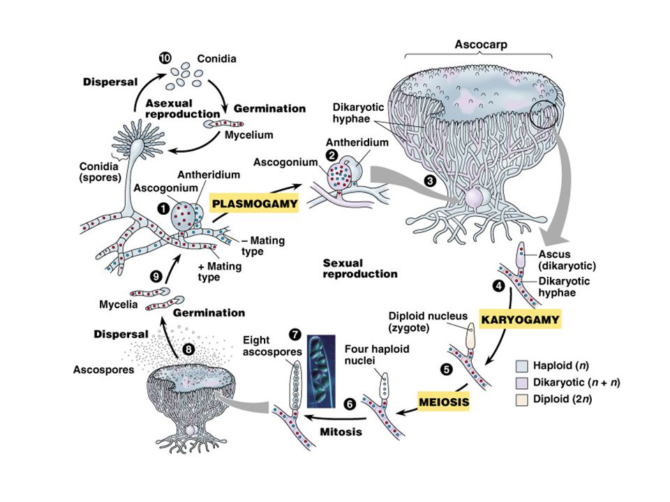
67. 5-79 Figure 5.12 Meiosis produces four haploid cells, termed spores
These are enclosed in a sac termed an ascus
Figure 5.12
5-79

68. The cells of a tetrad or octad are contained within a sac
In other words, the products of a single meiotic division are contained within one sac
This is a key feature that dramatically differs from sexual reproduction in animals and plants
In animals, for example
Oogenesis only produces a single functional egg
Spermatogenesis produces sperm that are mixed with millions of other sperm
Using a microscope, researchers can dissect asci and study the traits of each haploid spore
5-80
Copyright ©The McGraw-Hill Companies, Inc. Permission required for reproduction or display

69. Types of Tetrads or Octads
The arrangement of spores within an ascus varies from species to species
Unordered tetrads or octads
Ascus provides enough space for the spores to randomly mix together
Ordered tetrads or octads
Ascus is very tight, thereby preventing spores from randomly moving around
5-81
Copyright ©The McGraw-Hill Companies, Inc. Permission required for reproduction or display

70. 5-82 Tight ascus prevents mixing of spores
Ascus provides space for spores to randomly mix together
Mold
Yeast
Unicellular alga
Figure 5.13
5-82
Copyright ©The McGraw-Hill Companies, Inc. Permission required for reproduction or display

71. Ordered Tetrad Analysis
Ordered tetrads or octads have the following key feature
The position and order of spores within the ascus is determined by the divisions of meiosis and mitosis
This idea is schematically shown in Figure 5.13b
The example depicts ordered octad formation in Neurospora crassa
Spores that carry the A allele show orange pigmentation
Spores that carry the a (albino) allele are white
5-83
Copyright ©The McGraw-Hill Companies, Inc. Permission required for reproduction or display

72. Pairs of daughter cells are located next to each other
All eight cells are arranged in a linear, ordered fashion
Pairs of daughter cells are located next to each other
Figure 5.13
5-84
Copyright ©The McGraw-Hill Companies, Inc. Permission required for reproduction or display

73. 020
020. A linear, cylindrical, eight-spored ascus of Sordaria fimicola. Note ascosporogenesis (sexual reproduction in the Ascomycotina) involves the formation of ascospores, typically eight, by "free cell formation" within an ascus.

74. The genetic content of spores in ordered tetrads can be determined
This allows experimenters to map the distance between a single gene and the centromere
The logic of this mapping technique is based on the following features of meiosis
Centromeres of homologous chromosomes separate during meiosis I
Centromeres of sister chromatids separate during meiosis II
5-85
Copyright ©The McGraw-Hill Companies, Inc. Permission required for reproduction or display

75. 5-86 Figure 5.14 (a) No crossing over
Octad contains a linear arrangement of 4 haploid cells with the A allele which are adjacent to 4 with the a allele
This 4:4 arrangement of spores within the ascus is termed a first-division segregation (FDS) or an M1 pattern
Because the A and a alleles have segregated from each other after meiosis I
Figure 5.14 (a) No crossing over
5-86
Copyright ©The McGraw-Hill Companies, Inc. Permission required for reproduction or display

76. 5-87 Figure 5.14 (b) Single crossing over
These arrangement of spores are termed a second-division segregation (SDS) or M2 patterns
The A and a alleles do not segregate until meiosis II
Figure 5.14 (b) Single crossing over
5-87

77. The percentage of M2 asci can be used to calculate the map distance between the centromere and the gene of interest
5-88
Figure 5.15

78. (1/2) (Number of SDS asci) X 100 Map distance = Total number of asci
Therefore the chances of getting a 2:2:2:2 or 2:4:2 pattern depend on the distance between the gene of interest and the centromere
To calculate this distance, the experimenter must count the number of SDS asci, as well as the total number of asci
In SDS asci, only half of the spores are actually the product of a crossover
Therefore
(1/2) (Number of SDS asci)
X 100
Map distance =
Total number of asci
5-89
Copyright ©The McGraw-Hill Companies, Inc. Permission required for reproduction or display

79. Unordered Tetrad Analysis
Unicellular algae
Figure 5-18 The life cycle of Chlamydomonas. The diploid zygote (in the center) undergoes meiosis, producing [[p]][[p]] or [[p]][[p]] haploid cells that undergo mitosis, yielding vegetative colonies. Unfavorable conditions stimulate them to form isogametes, which fuse in fertilization, producing a zygote that repeats the cycle. Vegetative colonies are illustrated photographically.
Figure Copyright © 2006 Pearson Prentice Hall, Inc.

80. Unordered Tetrad Analysis
Unordered tetrads contain randomly arranged groups of spores
An experimenter can do a dihybrid cross and then determine the phenotypes of the spores
Such an analysis can determine if two genes are linked or assort independently
It can also be used to compute distance between two linked genes
5-90
Copyright ©The McGraw-Hill Companies, Inc. Permission required for reproduction or display

81. Unordered Tetrad Analysis
Consider a diploid yeast zygote with the genotype ura+ura-2 arg+arg-3
ura+ and arg+ = Normal alleles required for uracil and arginine biosynthesis, respectively
ura-2 and arg-3 = Defective alleles
Result in strains that require uracil and arginine in their growth medium
Figure 5.16 illustrates the assortment of the two genes in the unordered tetrad
5-91
Copyright ©The McGraw-Hill Companies, Inc. Permission required for reproduction or display

82. 5-92 Figure 5.16 PD ascus: contains 100% parental cells
T ascus: contains 50% parental cells and 50% recombinant cells
NPD ascus: contains 100% recombinant cells
5-92

83. If the two genes assort independently
The number of asci with a parental ditype is expected to equal the number with a nonparental ditype
Thus, 50% recombinant spores are produced
If the two genes are linked
The type of crossover between them determines what type of ascus is produced
No crossovers yield the parental ditype
Single crossovers produce the tetratype
Double crossovers can yield any of the three types
The actual type produced depends on the combination of chromatids that are involved
5-93
Copyright ©The McGraw-Hill Companies, Inc. Permission required for reproduction or display

84. Figure 5.17
5-94
Copyright ©The McGraw-Hill Companies, Inc. Permission required for reproduction or display

85. Figure 5.17
5-95

86. A more precise way to calculate map distance
As in conventional mapping, the map distance is calculated as the % of offspring that carry recombinant chromosomes
NPD + (1/2) (T)
Map distance =
X 100
Total number of asci
This calculation is fairly reliable over a short distance
However, over long distances it is not
Because it does not adequately account for double crossovers
A more precise way to calculate map distance
Single crossover tetrads +
(2) (Double crossover tetrads)
Map distance =
X 0.5 X 100
Total number of asci
Crossover tetrads also contain 50% nonrecombinant chromosomes
5-96
Copyright ©The McGraw-Hill Companies, Inc. Permission required for reproduction or display

87. So let’s take another look at Figure 5.17
For the equation to be useful, it needs to be related to the number of various types obtained by experimentation
So let’s take another look at Figure 5.17
The parental ditype (PD) and tetratype (T) are ambiguous
They can each be derived in two different ways
The nonparental ditype (NPD), however, is unambiguous
It can only be produced from a double crossover (DCO)
1/4 of all the double crossovers are nonparental ditypes
Therefore, DCO = 4 X NPD
But what about single crossovers (SCO)?
Notice that T asci can result from SCO or DCO
Since there are two kinds of T that are due to DCO
The actual number of T arising from DCO is 2NPD
So, T = SCO + 2NPD
Therefore, SCO = T – 2NPD
5-97
Copyright ©The McGraw-Hill Companies, Inc. Permission required for reproduction or display

88. Now we have accurate measures of both SCO and DCO
SCO = T – 2NPD and DCO = 4NPD
So, let’s substitute these values into our previous equation
Single crossover tetrads +
(2) (Double crossover tetrads)
Total number of asci
X 0.5 X 100
Map distance =
(T – 2NPD) + (2) (4NPD)
Map distance =
Total number of asci
X 0.5 X 100
T + 6NPD
Map distance =
Total number of asci
X 0.5 X 100
A more accurate measure of map distance because the equation considers both single- and double-crossovers
5-98
Copyright ©The McGraw-Hill Companies, Inc. Permission required for reproduction or display