Download presentation
Presentation is loading. Please wait.

1
Lecture 6 Sharpening Filters
The concept of sharpening filter First and second order derivatives Laplace filter Unsharp mask High boost filter Gradient mask Sharpening image with MatLab

2
Sharpening Spatial Filters
Department of Computer Engineering, CMU Sharpening Spatial Filters To highlight fine detail in an image or to enhance detail that has been blurred, either in error or as a natural effect of a particular method of image acquisition. Blurring vs. Sharpening Blurring/smooth is done in spatial domain by pixel averaging in a neighbors, it is a process of integration Sharpening is an inverse process, to find the difference by the neighborhood, done by spatial differentiation.

3
Department of Computer Engineering, CMU
Derivative operator The strength of the response of a derivative operator is proportional to the degree of discontinuity of the image at the point at which the operator is applied. Image differentiation enhances edges and other discontinuities (noise) deemphasizes area with slowly varying gray-level values.
 deemphasizes area with slowly varying gray-level values.")
4
Sharpening edge by First and second order derivatives
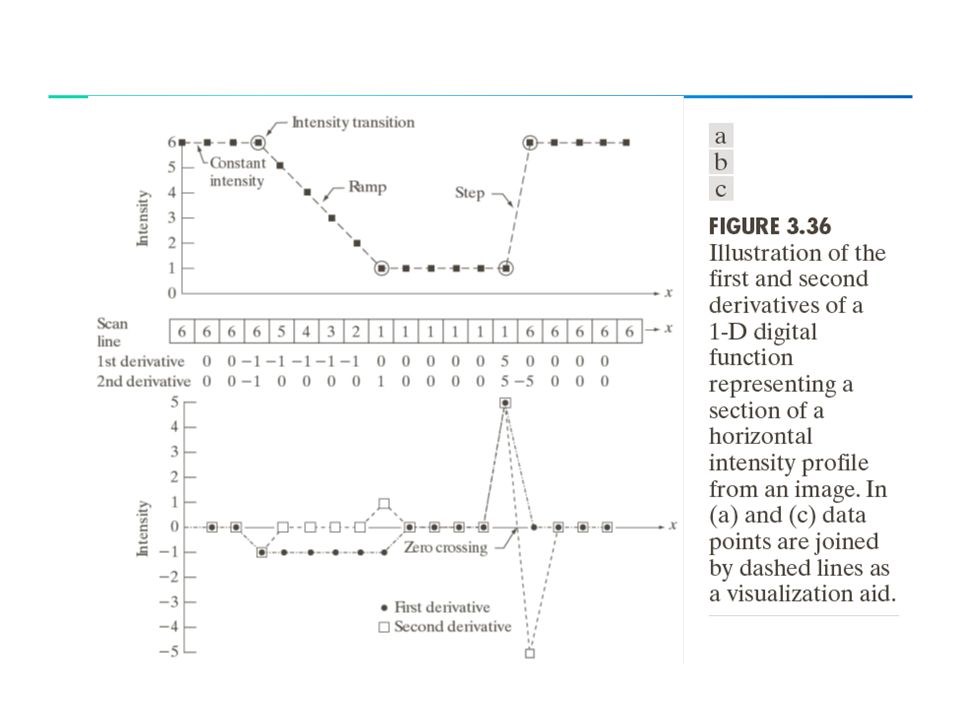
Department of Computer Engineering, CMU Sharpening edge by First and second order derivatives Intensity function f = First derivative f’ = Second-order derivative f’’ = f- f’’ = f’ f f’’ f-f’’

5
First and second order difference of 1D
Department of Computer Engineering, CMU First and second order difference of 1D The basic definition of the first-order derivative of a one-dimensional function f(x) is the difference The second-order derivative of a one-dimensional function f(x) is the difference
 is the difference. The second-order derivative of a one-dimensional function f(x) is the difference.")
7
First and Second-order derivative of 2D
Department of Computer Engineering, CMU First and Second-order derivative of 2D when we consider an image function of two variables, f(x, y), at which time we will dealing with partial derivatives along the two spatial axes. (linear operator) Laplacian operator (non-linear) Gradient operator
, at which time we will dealing with partial derivatives along the two spatial axes. (linear operator) Laplacian operator (non-linear) Gradient operator.")
8
Discrete form of Laplacian
Department of Computer Engineering, CMU Discrete form of Laplacian from

9
Department of Computer Engineering, CMU
Result Laplacian mask

10
Laplacian mask implemented an extension of diagonal neighbors

11
Other implementation of Laplacian masks
give the same result, but we have to keep in mind that when combining (add / subtract) a Laplacian-filtered image with another image.
 a Laplacian-filtered image with another image.")
12
Effect of Laplacian Operator
Department of Computer Engineering, CMU Effect of Laplacian Operator as it is a derivative operator, it highlights gray-level discontinuities in an image it deemphasizes regions with slowly varying gray levels tends to produce images that have grayish edge lines and other discontinuities, all superimposed on a dark, featureless background.

13
Correct the effect of featureless background
easily by adding the original and Laplacian image. be careful with the Laplacian filter used if the center coefficient of the Laplacian mask is negative if the center coefficient of the Laplacian mask is positive

14
Department of Computer Engineering, CMU
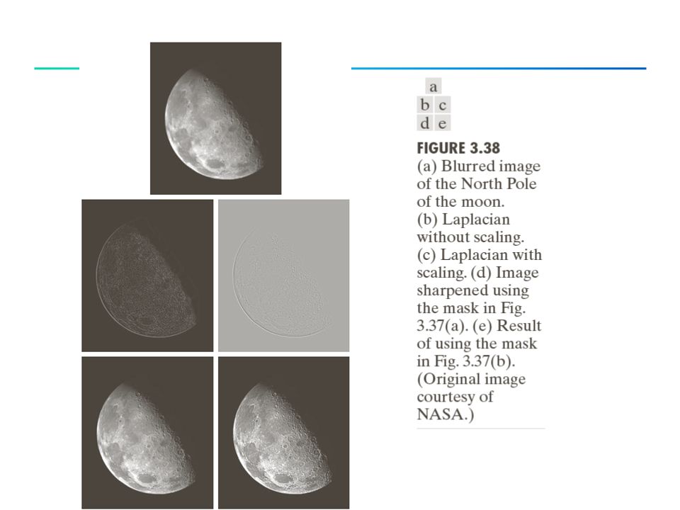
Example a). image of the North pole of the moon b). Laplacian-filtered image with c). Laplacian image scaled for display purposes d). image enhanced by addition with original image 1 -8
. image of the North pole of the moon. b). Laplacian-filtered image with. c). Laplacian image scaled for display purposes. d). image enhanced by addition with original image")
15
Mask of Laplacian + addition
Department of Computer Engineering, CMU Mask of Laplacian + addition to simply the computation, we can create a mask which do both operations, Laplacian Filter and Addition the original image.

16
Mask of Laplacian + addition
Department of Computer Engineering, CMU Mask of Laplacian + addition -1 5

17
Example

18
Department of Computer Engineering, CMU
Note 1 -1 4 -1 5 + = 1 -1 8 -1 9 + =

19
Unsharp masking sharpened image = original image – blurred image
to subtract a blurred version of an image produces sharpening output image.

20
Unsharp mask

22
Department of Computer Engineering, CMU
High-boost filtering generalized form of Unsharp masking A 1

23
High-boost filtering if we use Laplacian filter to create sharpen image fs(x,y) with addition of original image
 with addition of original image.")
24
Department of Computer Engineering, CMU
High-boost Masks A 1 if A = 1, it becomes “standard” Laplacian sharpening

25
Department of Computer Engineering, CMU
Example

26
Gradient Operator first derivatives are implemented using the magnitude of the gradient. the magnitude becomes nonlinear commonly approx.

27
Department of Computer Engineering, CMU
Gradient Mask z1 z2 z3 z4 z5 z6 z7 z8 z9 simplest approximation, 2x2

28
Gradient Mask z1 z2 z3 z4 z5 z6 z7 z8 z9
Roberts cross-gradient operators, 2x2

29
Department of Computer Engineering, CMU
z1 z2 z3 z4 z5 z6 z7 z8 z9 Gradient Mask Sobel operators, 3x3 the weight value 2 is to achieve smoothing by giving more important to the center point

30
Example

31
Example of Combining Spatial Enhancement Methods
want to sharpen the original image and bring out more skeletal detail. problems: narrow dynamic range of gray level and high noise content makes the image difficult to enhance

32
Example of Combining Spatial Enhancement Methods
solve : Laplacian to highlight fine detail gradient to enhance prominent edges gray-level transformation to increase the dynamic range of gray levels

33
Department of Computer Engineering, CMU

Similar presentations
 dr. Andrea Fuster dr. Anna Vilanova Prof.dr.ir. Marcel Breeuwer Filtering.>")

>")


