1. Local Enhancement Histogram processing methods are global processing, in the sense that pixels are modified by a transformation function based on the gray-level content of an entire image. Histogram processing methods are global processing, in the sense that pixels are modified by a transformation function based on the gray-level content of an entire image. Sometimes, we may need to enhance details over small areas in an image, which is called a local enhancement. Sometimes, we may need to enhance details over small areas in an image, which is called a local enhancement.

2. Local Enhancement define a square or rectangular neighborhood and move the center of this area from pixel to pixel. define a square or rectangular neighborhood and move the center of this area from pixel to pixel. at each location, the histogram of the points in the neighborhood is computed and either histogram equalization or histogram specification transformation function is obtained. at each location, the histogram of the points in the neighborhood is computed and either histogram equalization or histogram specification transformation function is obtained. another approach used to reduce computation is to utilize nonoverlapping regions, but it usually produces an undesirable checkerboard effect. another approach used to reduce computation is to utilize nonoverlapping regions, but it usually produces an undesirable checkerboard effect. a)Original image (slightly blurred to reduce noise) b)global histogram equalization (enhance noise & slightly increase contrast but the construction is not changed) c)local histogram equalization using 7x7 neighborhood (reveals the small squares inside larger ones of the original image. (a)(b)(c)

3. Explain the result in c) Basically, the original image consists of many small squares inside the larger dark ones. Basically, the original image consists of many small squares inside the larger dark ones. However, the small squares were too close in gray level to the larger ones, and their sizes were too small to influence global histogram equalization significantly. However, the small squares were too close in gray level to the larger ones, and their sizes were too small to influence global histogram equalization significantly. So, when we use the local enhancement technique, it reveals the small areas. So, when we use the local enhancement technique, it reveals the small areas. Note also the finer noise texture is resulted by the local processing using relatively small neighborhoods. Note also the finer noise texture is resulted by the local processing using relatively small neighborhoods.

4. Enhancement using Arithmetic/Logic Operations Arithmetic/Logic operations perform on pixel by pixel basis between two or more images Arithmetic/Logic operations perform on pixel by pixel basis between two or more images except NOT operation which perform only on a single image except NOT operation which perform only on a single image

5. Logic Operations Logic operation performs on gray- level images, the pixel values are processed as binary numbers Logic operation performs on gray- level images, the pixel values are processed as binary numbers light represents a binary 1, and dark represents a binary 0 light represents a binary 1, and dark represents a binary 0 NOT operation = negative transformation NOT operation = negative transformation

6. Example of AND Operation original imageAND image mask result of AND operation

7. Example of OR Operation original imageOR image mask result of OR operation

8. Image Subtraction g(x,y) = f(x,y) – h(x,y) enhancement of the differences between images enhancement of the differences between images

9. Image Subtraction a). original fractal image a). original fractal image b). result of setting the four lower-order bit planes to zero b). result of setting the four lower-order bit planes to zero refer to the bit-plane slicing the higher planes contribute significant detail the lower planes contribute more to fine detail image b). is nearly identical visually to image a), with a very slightly drop in overall contrast due to less variability of the gray-level values in the image. c). difference between a). and b). (nearly black) c). difference between a). and b). (nearly black) d). histogram equalization of c). (perform contrast stretching transformation) d). histogram equalization of c). (perform contrast stretching transformation)abcd

14. Spatial Filtering use filter (can also be called as mask/kernel/template or window) use filter (can also be called as mask/kernel/template or window) the values in a filter subimage are referred to as coefficients, rather than pixel. the values in a filter subimage are referred to as coefficients, rather than pixel. our focus will be on masks of odd sizes, e.g. 3x3, 5x5,… our focus will be on masks of odd sizes, e.g. 3x3, 5x5,…

16. Spatial Filtering Process simply move the filter mask from point to point in an image. simply move the filter mask from point to point in an image. at each point (x,y), the response of the filter at that point is calculated using a predefined relationship. at each point (x,y), the response of the filter at that point is calculated using a predefined relationship.

17. Smoothing Spatial Filters used for blurring and for noise reduction used for blurring and for noise reduction blurring is used in preprocessing steps, such as blurring is used in preprocessing steps, such as removal of small details from an image prior to object extractionremoval of small details from an image prior to object extraction bridging of small gaps in lines or curvesbridging of small gaps in lines or curves noise reduction can be accomplished by blurring with a linear filter and also by a nonlinear filter noise reduction can be accomplished by blurring with a linear filter and also by a nonlinear filter

18. Smoothing Linear Filters output is simply the average of the pixels contained in the neighborhood of the filter mask. output is simply the average of the pixels contained in the neighborhood of the filter mask. called averaging filters or lowpass filters. called averaging filters or lowpass filters.

19. Smoothing Linear Filters replacing the value of every pixel in an image by the average of the gray levels in the neighborhood will reduce the “sharp” transitions in gray levels. replacing the value of every pixel in an image by the average of the gray levels in the neighborhood will reduce the “sharp” transitions in gray levels. sharp transitions sharp transitions random noise in the imagerandom noise in the image edges of objects in the imageedges of objects in the image thus, smoothing can reduce noises (desirable) and blur edges (undesirable) thus, smoothing can reduce noises (desirable) and blur edges (undesirable)

20. 3x3 Smoothing Linear Filters box filterweighted average the center is the most important and other pixels are inversely weighted as a function of their distance from the center of the mask

21. Weighted average filter the basic strategy behind weighting the center point the highest and then reducing the value of the coefficients as a function of increasing distance from the origin is simply an attempt to reduce blurring in the smoothing process. the basic strategy behind weighting the center point the highest and then reducing the value of the coefficients as a function of increasing distance from the origin is simply an attempt to reduce blurring in the smoothing process.

22. Example a). original image 500x500 pixel a). original image 500x500 pixel b). - f). results of smoothing with square averaging filter masks of size n = 3, 5, 9, 15 and 35, respectively. b). - f). results of smoothing with square averaging filter masks of size n = 3, 5, 9, 15 and 35, respectively. Note: Note: big mask is used to eliminate small objects from an image. the size of the mask establishes the relative size of the objects that will be blended with the background.abcd ef

23. Order-Statistics Filters (Nonlinear Filters) the response is based on ordering (ranking) the pixels contained in the image area encompassed by the filter the response is based on ordering (ranking) the pixels contained in the image area encompassed by the filter example example median filter : R = median{z k |k = 1,2,…,n x n}median filter : R = median{z k |k = 1,2,…,n x n} max filter : R = max{z k |k = 1,2,…,n x n}max filter : R = max{z k |k = 1,2,…,n x n} min filter : R = min{z k |k = 1,2,…,n x n}min filter : R = min{z k |k = 1,2,…,n x n} note: n x n is the size of the mask note: n x n is the size of the mask

24. Median Filters replaces the value of a pixel by the median of the gray levels in the neighborhood of that pixel (the original value of the pixel is included in the computation of the median) replaces the value of a pixel by the median of the gray levels in the neighborhood of that pixel (the original value of the pixel is included in the computation of the median) quite popular because for certain types of random noise (impulse noise  salt and pepper noise), they provide excellent noise-reduction capabilities, with considering less blurring than linear smoothing filters of similar size. quite popular because for certain types of random noise (impulse noise  salt and pepper noise), they provide excellent noise-reduction capabilities, with considering less blurring than linear smoothing filters of similar size.

26. 26 Example : Median Filters

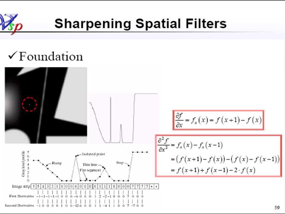
27. 27 Sharpening Spatial Filters to highlight fine detail in an image to highlight fine detail in an image or to enhance detail that has been blurred, either in error or as a natural effect of a particular method of image acquisition. or to enhance detail that has been blurred, either in error or as a natural effect of a particular method of image acquisition.

28. 28 Blurring vs. Sharpening as we know that blurring can be done in spatial domain by pixel averaging in a neighbors as we know that blurring can be done in spatial domain by pixel averaging in a neighbors since averaging is analogous to integration since averaging is analogous to integration thus, we can guess that the sharpening must be accomplished by spatial differentiation. thus, we can guess that the sharpening must be accomplished by spatial differentiation.

29. 29 Derivative operator the strength of the response of a derivative operator is proportional to the degree of discontinuity of the image at the point at which the operator is applied. the strength of the response of a derivative operator is proportional to the degree of discontinuity of the image at the point at which the operator is applied. thus, image differentiation thus, image differentiation enhances edges and other discontinuities (noise)enhances edges and other discontinuities (noise) deemphasizes area with slowly varying gray- level values.deemphasizes area with slowly varying gray- level values.

30. 30 First-order derivative a basic definition of the first-order derivative of a one-dimensional function f(x) is the difference a basic definition of the first-order derivative of a one-dimensional function f(x) is the difference

31. 31 Second-order derivative similarly, we define the second-order derivative of a one-dimensional function f(x) is the difference similarly, we define the second-order derivative of a one-dimensional function f(x) is the difference

32. Response of First and Second order derivatives Response of first order derivative is: zero in flat segments (area of constant grey values) zero in flat segments (area of constant grey values) Non zero at the onset of a grey level step or ramp Non zero at the onset of a grey level step or ramp Non zero along ramps Non zero along ramps Response of second order derivative is: Zero in flat areas Zero in flat areas Non zero at the onset of a grey level step or ramp Non zero at the onset of a grey level step or ramp Zero along ramps of constant slope Zero along ramps of constant slope

34. First and Second-order derivative of f(x,y) when we consider an image function of two variables, f(x,y), at which time we will dealing with partial derivatives along the two spatial axes. when we consider an image function of two variables, f(x,y), at which time we will dealing with partial derivatives along the two spatial axes. (linear operator) Laplacian operator Gradient operator

35. Discrete Form of Laplacian from yield,

36. Result Laplacian mask

37. Laplacian mask implemented an extension of diagonal neighbors

38. Other implementation of Laplacian masks give the same result, but we have to keep in mind that when combining (add / subtract) a Laplacian-filtered image with another image.

39. Effect of Laplacian Operator as it is a derivative operator, as it is a derivative operator, it highlights gray-level discontinuities in an imageit highlights gray-level discontinuities in an image it deemphasizes regions with slowly varying gray levelsit deemphasizes regions with slowly varying gray levels tends to produce images that have tends to produce images that have grayish edge lines and other discontinuities, all superimposed on a dark,grayish edge lines and other discontinuities, all superimposed on a dark, featureless background.featureless background.

40. Correct the effect of featureless background easily by adding the original and Laplacian image. easily by adding the original and Laplacian image. be careful with the Laplacian filter used be careful with the Laplacian filter used if the center coefficient of the Laplacian mask is negative if the center coefficient of the Laplacian mask is positive

41. Example a). image of the North pole of the moon a). image of the North pole of the moon b). Laplacian-filtered image with b). Laplacian-filtered image with c). Laplacian image scaled for display purposes c). Laplacian image scaled for display purposes d). image enhanced by addition with original image d). image enhanced by addition with original image1111-81 111

42. Mask of Laplacian + addition to simply the computation, we can create a mask which do both operations, Laplacian Filter and Addition the original image. to simply the computation, we can create a mask which do both operations, Laplacian Filter and Addition the original image.

43. Mask of Laplacian + addition 005 00

44. Example

45. Note 005 00 000010 000 = +004 00 009 00 000010 000 = +008 00

46. Unsharp masking to subtract a blurred version of an image produces sharpening output image. to subtract a blurred version of an image produces sharpening output image. sharpened image = original image – blurred image

47. High-boost filtering generalized form of Unsharp masking generalized form of Unsharp masking A  1 A  1

48. High-boost filtering if we use Laplacian filter to create sharpen image f s (x,y) with addition of original image if we use Laplacian filter to create sharpen image f s (x,y) with addition of original image

49. High-boost filtering yields yields if the center coefficient of the Laplacian mask is negative if the center coefficient of the Laplacian mask is positive

50. High-boost Masks A  1 A  1 if A = 1, it becomes “standard” Laplacian sharpening if A = 1, it becomes “standard” Laplacian sharpening

51. Example

52. Gradient Operator first derivatives are implemented using the magnitude of the gradient. first derivatives are implemented using the magnitude of the gradient. the magnitude becomes nonlinear commonly approx.

53. Gradient Mask simplest approximation, 2x2 simplest approximation, 2x2 z1z1z1z1 z2z2z2z2 z3z3z3z3 z4z4z4z4 z5z5z5z5 z6z6z6z6 z7z7z7z7 z8z8z8z8 z9z9z9z9

54. Gradient Mask Sobel operators, 3x3 Sobel operators, 3x3 z1z1z1z1 z2z2z2z2 z3z3z3z3 z4z4z4z4 z5z5z5z5 z6z6z6z6 z7z7z7z7 z8z8z8z8 z9z9z9z9 the weight value 2 is to achieve smoothing by giving more important to the center point

55. Note the summation of coefficients in all masks equals 0, indicating that they would give a response of 0 in an area of constant gray level. the summation of coefficients in all masks equals 0, indicating that they would give a response of 0 in an area of constant gray level.

56. Example

57. Example of Combining Spatial Enhancement Methods want to sharpen the original image and bring out more skeletal detail. want to sharpen the original image and bring out more skeletal detail. problems: narrow dynamic range of gray level and high noise content makes the image difficult to enhance problems: narrow dynamic range of gray level and high noise content makes the image difficult to enhance

58. Example of Combining Spatial Enhancement Methods solve : solve : 1.Laplacian to highlight fine detail 2.gradient to enhance prominent edges 3.gray-level transformation to increase the dynamic range of gray levels

61. Image Enhancement in the Frequency Domain

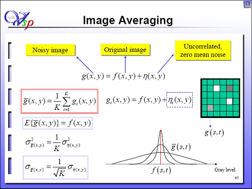
62. Fourier Series Any function that periodically repeats itself can be expressed as the sum of sines and/or cosines of different frequencies, each multiplied by a different coefficients. This sum is called a Fourier series.

63. Fourier Series

64. Fourier Transform A function that is not periodic but the area under its curve is finite can be expressed as the integral of sines and/or cosines multiplied by a weighing function. The formulation in this case is Fourier transform.

65. The One-Dimensional Fourier Transform and its Inverse The fourier transform F(u) : The fourier transform F(u) : The inverse Fourier transform f(x) : The inverse Fourier transform f(x) : Two variables Fourier transform F(u, v) : Two variables Fourier transform F(u, v) : The inverse transform f(x, y) : The inverse transform f(x, y) :

66. The One-Dimensional Fourier Transform and its Inverse The discrete Fourier Transform F(u) : The discrete Fourier Transform F(u) : The inverse DFT : The inverse DFT : Apply euler ’ s formula : Apply euler ’ s formula :

67. The One-Dimensional Fourier Transform and its Inverse F(u) in polar coordinates : F(u) in polar coordinates :

68. The One-Dimensional Fourier Transform and its Inverse

69. The two dimensional DFT and its Inverse The discrete fourier transform of a function f(x,y) of size M x N : The discrete fourier transform of a function f(x,y) of size M x N : The inverse Fourier transform : The inverse Fourier transform :

70. The two dimensional DFT and its Inverse In the polar coordinate In the polar coordinate

71. The two dimensional DFT and its Inverse DFT corresponding (u,v)=(0,0) DFT corresponding (u,v)=(0,0) If f(x,y) is real, its Fourier transform is conjugate symmetric If f(x,y) is real, its Fourier transform is conjugate symmetric The spectrum of the Fourier transform is symmetric The spectrum of the Fourier transform is symmetric

72. The two dimensional DFT and its Inverse

73. Basics of filtering in the frequency domain 1. Multiply the input image by to center the transform 2. Compute F(u,v), by the DFT of the image from (1) 3. Multiply F(u,v) by a filter function H(u,v) 4. Compute the inverse DFT of the result in (3) 5. Obtain the real part of the result in (4) 6. Multiply the result in (5) by

74. Basics of filtering in the frequency domain

75. Some basic filters and their properties

76. Lowpass filter : less sharp (Smoothing) Lowpass filter : less sharp (Smoothing) Highpass filter : less gray-level variation and emphasized edges (Sharpening) Highpass filter : less gray-level variation and emphasized edges (Sharpening)

77. Correspondence between Filtering in the Spatial and Frequency Domains The convolution theorem : The convolution theorem : The impulse response : The impulse response :

78. Correspondence between Filtering in the Spatial and Frequency Domains The Fourier transform of a unit impulse function The Fourier transform of a unit impulse function Let Let

79. Correspondence between Filtering in the Spatial and Frequency Domains Gaussian functions : Gaussian functions :

80. Correspondence between Filtering in the Spatial and Frequency Domains

81. Smoothing Frequency-Domain Filters Ideal Ideal Butterworth Butterworth Gaussian Gaussian

82. Ideal lowpass filter

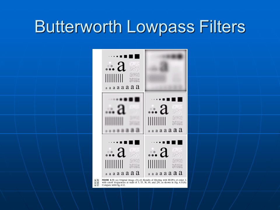
87. Butterworth Lowpass Filters When D(u,v)=, H(u,v)=0.5 When D(u,v)=, H(u,v)=0.5

88. Butterworth Lowpass Filters

91. Gaussian Lowpass filter let let

92. Gaussian Lowpass filter

94. Sharpening Frequency Domain Filters Ideal Ideal Butterworth Butterworth Gaussian Gaussian

95. Sharpening Frequency Domain Filters

96. Ideal Highpass Filters

97. Ideal highpass filter

98. Butterworth Highpass Filters

99. Gaussian Highpass Filters

100. The Laplacian in the Frequency Domain

103. Unsharp Masking, High-Boost Filtering, and High-Frequency Emphasis Filtering Unsharp masking : Unsharp masking : High-Boost filtering : High-Boost filtering : High-Frequency Emphasis Filtering High-Frequency Emphasis Filtering

104. Unsharp Masking, High-Boost Filtering, and High-Frequency Emphasis Filtering