Download presentation
Presentation is loading. Please wait.

1
Digital Image Processing In The Name Of God Digital Image Processing Lecture3: Image enhancement M. Ghelich Oghli By: M. Ghelich Oghli E-mail: m.g31_mesu@yahoo.com Fall 2012

2
Image Enhancement The principle Objective of enhancement is to process an image so that the result is more suitable than the original image for specific application Purpose Image enhancement for human reception Image Enhancement for machine automation Category Spatial domain Frequency domain

3
g(x,y)=T(f(x,y)) g(x,y,k)=T(f(x,y,k)) where g(x,y) is output image f(x,y) is input image x,y are spatial index k is temporal index Gray Level Transformation or point processing mm nn U[M×N] V[M×N]
![g(x,y)=T(f(x,y)) g(x,y,k)=T(f(x,y,k)) where g(x,y) is output image f(x,y) is input image x,y are spatial index k is temporal index Gray Level Transformation or point processing mm nn U[M×N] V[M×N]](http://images.slideplayer.com/15/4512089/slides/slide_3.jpg "g(x,y)=T(f(x,y)) g(x,y,k)=T(f(x,y,k)) where g(x,y) is output image f(x,y) is input image x,y are spatial index k is temporal index Gray Level Transformation or point processing mm nn U[M×N] V[M×N]")
4
Applying spatial domain filter (Sliding windows) AMAM
 AMAM")
5
Fig 3.2 Gray Level Transformation a) contrast enhancement b) thresholding
 contrast enhancement b) thresholding")
6
Some Useful Gray level (intensity) Transformation
 Transformation")
7
Log Transform

8
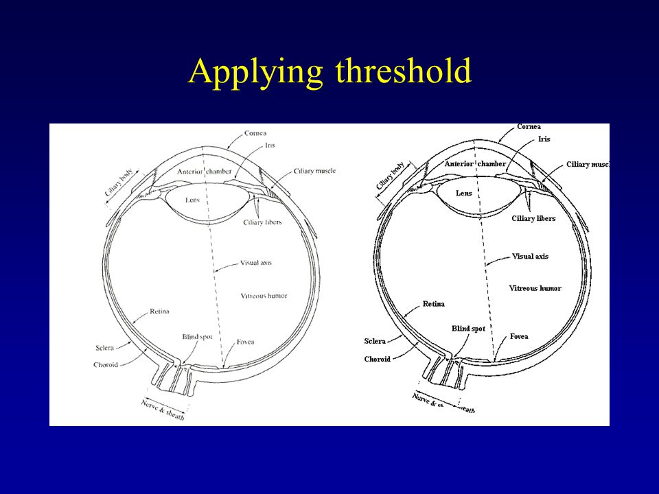
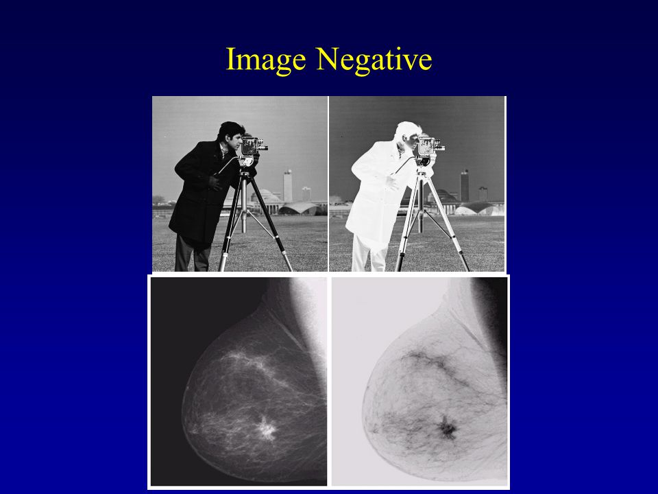
Image Negative Image intensity is in the range of [0, L-1] S=L-1-r Some Useful Gray level (intensity) Transformation Applying threshold
![Image Negative Image intensity is in the range of [0, L-1] S=L-1-r Some Useful Gray level (intensity) Transformation Applying threshold](http://images.slideplayer.com/15/4512089/slides/slide_8.jpg "Image Negative Image intensity is in the range of [0, L-1] S=L-1-r Some Useful Gray level (intensity) Transformation Applying threshold")
10
Image Negative

12
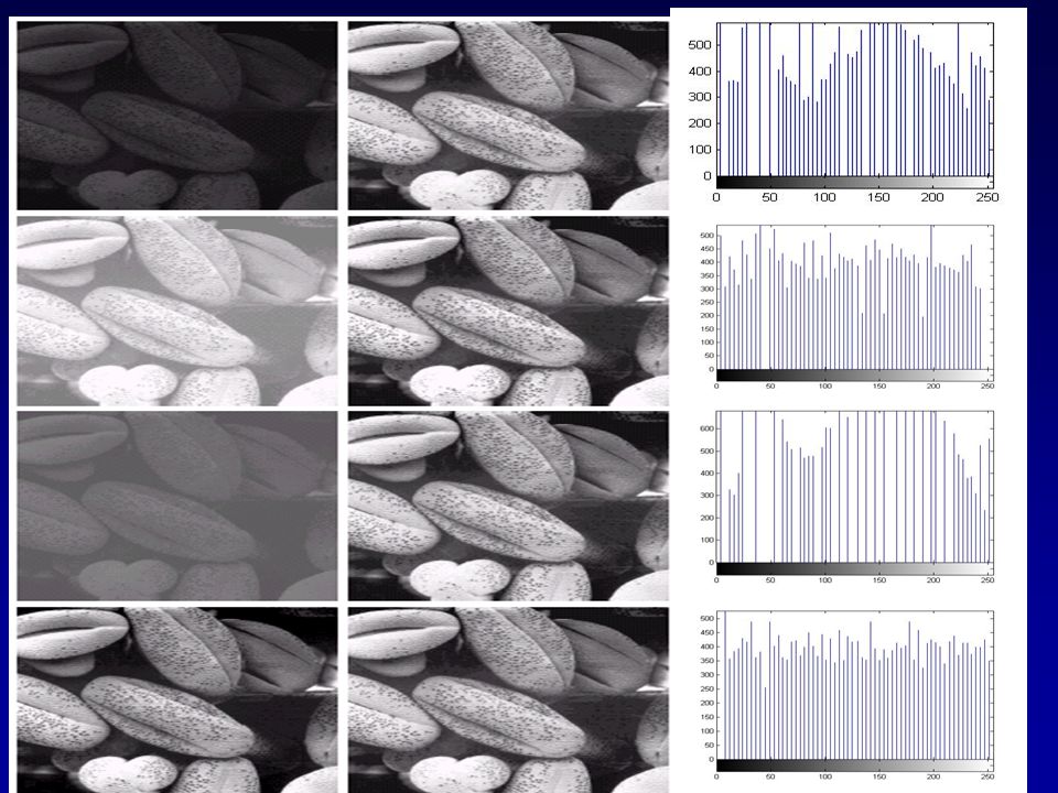
Gamma Correction

13
Gamma correction applied to forest picture(γ=0.5)
")
14
Gamma Correction

15
Histogram Processing The histogram of a digital image with gray levels from 0 to L-1 is a discrete function h(r k )=n k, where: r k is the kth gray level n k is the Number of pixels in the image with that gray level n is the total number of pixels in the image k = 0, 1, 2, …, L-1 Normalized histogram: p(r k )=n k /n –sum of all components = 1
=n k, where: r k is the kth gray level n k is the Number of pixels in the image with that gray level n is the total number of pixels in the image k = 0, 1, 2, …, L-1 Normalized histogram: p(r k )=n k /n –sum of all components = 1")
16
Dark image Bright image Histogram for different images

17
Low contrast image High contrast image Histogram for different images

18
Histogram Processing The shape of the histogram of an image does provide useful info about the possibility for contrast enhancement. Types of processing: Histogram equalization Histogram matching (specification) Local enhancement
 Local enhancement.")
19
Histogram Equalization Method Determine and Transformation function that seeks to produce an output image that has uniform histogram. S=T( r )0≤ r ≤1 Transformation Function a)T(r) is single-valued and monotonically increasing the interval 0≤ r ≤1 b)0≤T(r)≤1for 0≤ r ≤1
0≤ r ≤1 Transformation Function a)T(r) is single-valued and monotonically increasing the interval 0≤ r ≤1 b)0≤T(r)≤1for 0≤ r ≤1.")
20
Histogram Equalization

21
Histogram equalization(HE) results are similar to contrast stretching but offer the advantage of full automation, since HE automatically determines a transformation function to produce a new image with a uniform histogram.
 results are similar to contrast stretching but offer the advantage of full automation, since HE automatically determines a transformation function to produce a new image with a uniform histogram.")
23
Noise Images are corrupted by random variations in intensity values called noise due to non-perfect camera acquisition or environmental conditions. Assumptions: –Additive noise: a random value is added at each pixel –White noise: The value at a point is independent on the value at any other point.

24
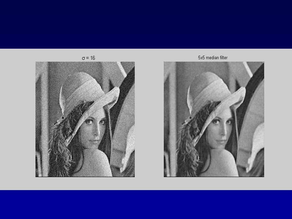
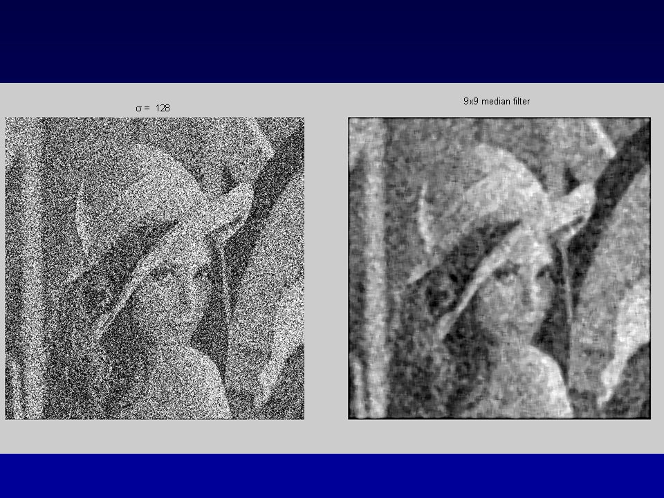
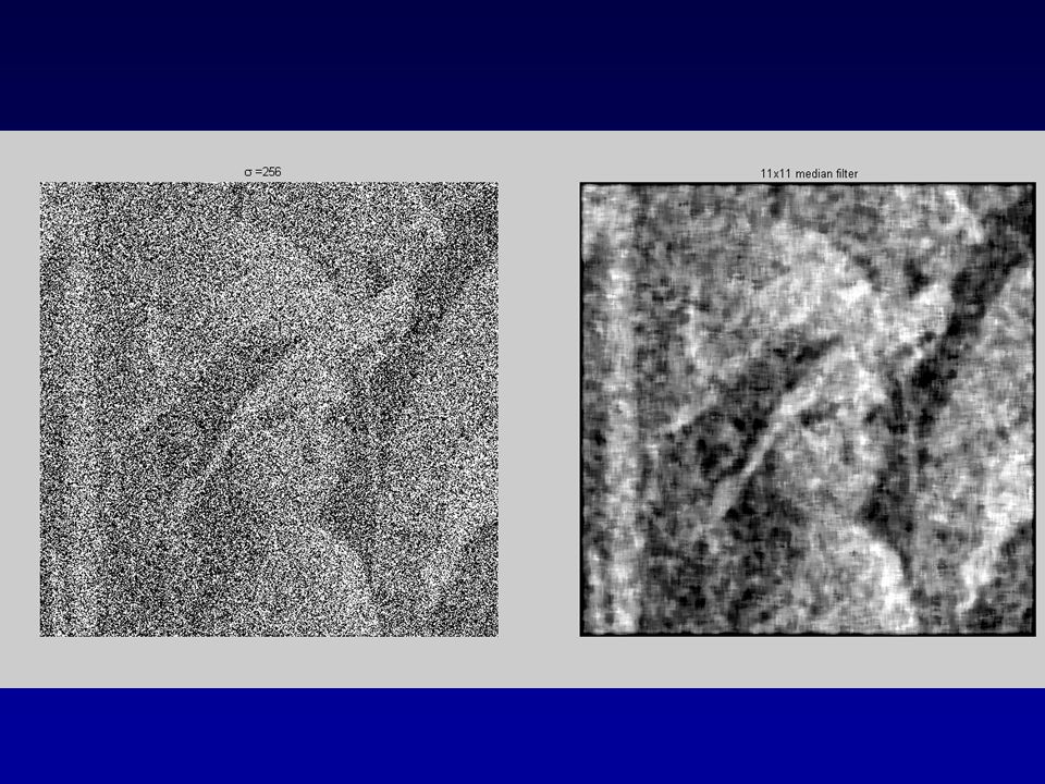
Salt and pepper noise random occurrences of both black and white intensity values are specified by noise density Impulse noise: random occurrences of white intensity values are specified by noise density Common Types of Noise

25
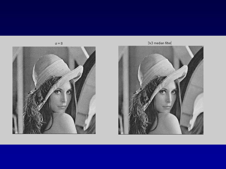
Gaussian noise: impulse noise but its intensity values are drawn from a Gaussian distribution models sensor noise (due to camera electronics) are specified by noise mean and variance or dB
 are specified by noise mean and variance or dB")
26
Examples of Noisy Images

27
Spatial Filtering

28
a=(m-1)/2 and b=(n-1)/2, m and n (odd numbers) For x=0,1,…,M-1 and y=0,1,…,N-1 Also called convolution (primarily in the frequency domain)
/2 and b=(n-1)/2, m and n (odd numbers) For x=0,1,…,M-1 and y=0,1,…,N-1 Also called convolution (primarily in the frequency domain)")
29
Spatial Filtering Another representation

30
Original Spatial Filtering

36
Linear Filters is filtering in which the value of an output pixel is a linear combination of the values of the pixels in the input pixel’s neighborhood Nonlinear Filter use pixel neighborhoods but do not explicitly use coefficients.

37
Spatial Filtering Low-pass filters eliminate or attenuate high frequency components in the frequency domain (sharp image details), and result in image blurring. High-pass filters attenuate or eliminate low-frequency components (resulting in sharpening edges and other sharp details). Band-pass filters remove selected frequency regions between low and high frequencies (for image restoration, not enhancement).
. Band-pass filters remove selected frequency regions between low and high frequencies (for image restoration, not enhancement)..")
38
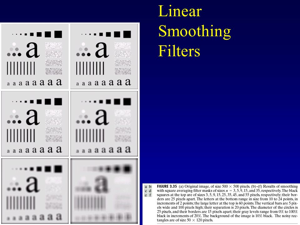
Linear Smoothing Filters Also are referred to averaging filter weighted averaging filter lowpass filter Results in blurring (removal of small details prior to large object extraction, bridging small gaps in lines) noise reduction.
 noise reduction.")
39
Linear Smoothing Filters

42
Order Statistic Filters

43
Sharpening Filters To highlight fine detail or to enhance blurred detail. –smoothing ~ integration –sharpening ~ differentiation Categories of sharpening filters: –Derivative operators –Basic highpass spatial filtering –High-boost filtering

44
The Gradient Non-isotropic Its magnitude (often call the gradient) is isotropic Computations is not trivial for whole image Reducing Computation Overhead
 is isotropic Computations is not trivial for whole image Reducing Computation Overhead")
45
The Gradient

46
The Uses of Gradient for Edge Detection

47
Digital Function Derivatives First derivative: –0 in constant gray segments –Non-zero at the onset of steps or ramps –Non-zero along ramps –Produce thicker edges in an image Second derivative: –0 in constant gray segments –Non-zero at the onset and end of steps or ramps –0 along ramps of constant slope. –Have stronger response to fine detail

48
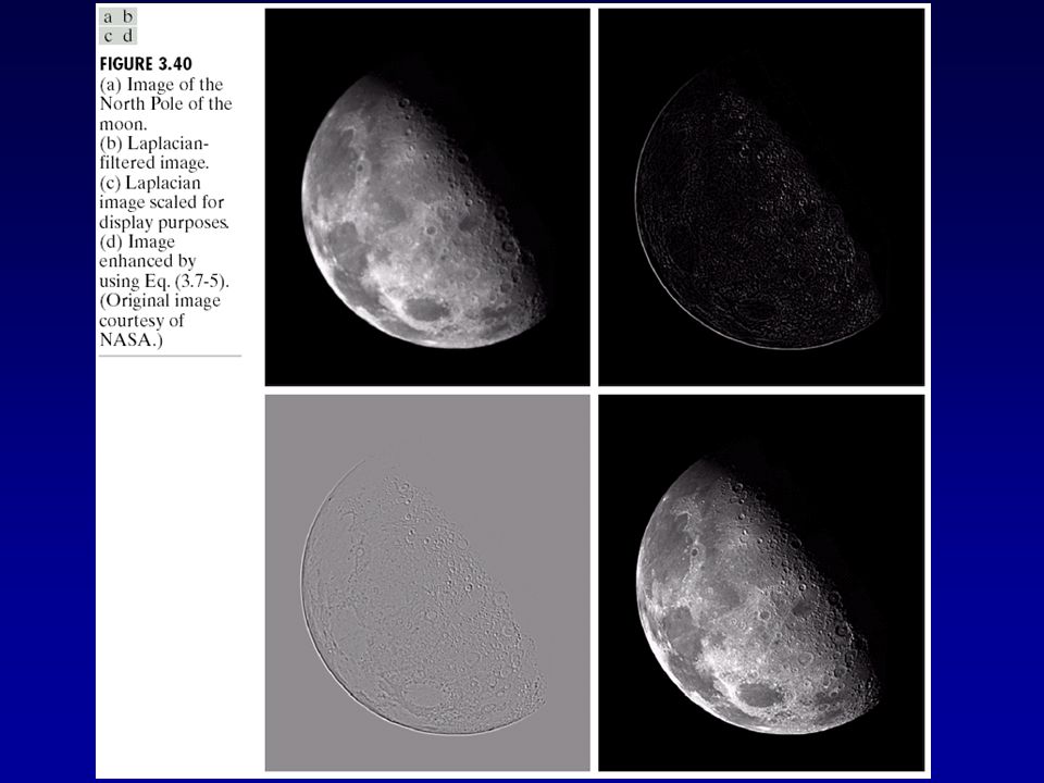
Laplacian Digital implementation: Two definitions of Laplacian: one is the negative of the other Accordingly, to recover background features: I: if the center of the mask is negative II: if the center of the mask is positive

49
Laplacian

Similar presentations


>")


=nk, where: rk is the kth gray level nk.>")


 operations are modeled as a linear system Linear System δ(x,y) h(x,y)>")


