Download presentation
Presentation is loading. Please wait.

1
Microsoft Office XP Microsoft Excel

2
Microsoft Office XP Microsoft Excel
Entering Text and Numbers Formatting Text and Performing Mathematical Calculations Numbers and Mathematical Calculations Creating Charts

3
Entering Text and Numbers
Start > Program > Microsoft Office > Microsoft Office Excel

4
Entering Text and Numbers
The Title Bar The Menu Bar

5
Toolbars The Standard Toolbar The Formatting Toolbar

6
Show full menus Point to the word Tools, which is located on the menu bar. Click your left mouse button. Press the down arrow until customize is highlighted. Press Enter. Choose the Options Tab by clicking on it. If Always Show Full Menus does not have a check mark in it, click in the Always Show Full Menus box. Click Close to close the dialog box.

7
Show full menus

8
Show full menus

9
Show full menus

10
Worksheets

11
The Formula Bar If the Formula bar is turned on, the cell address displays in the Name box on the left side of the Formula bar. Cell entries display on the right side of the Formula bar. Before proceeding, make sure the Formula bar is turned on.

12
Selecting Cells

13
Selecting Cells Go to Specific Cell By pressing the F8 key
Using the shift key Go to Specific Cell Go to -- F5 Go to -- Ctrl-G

14
Wrapping Text

15
Wrapping Text Return to the Cell
Choose Format > Cells from the menu. Choose the Alignment tab. Click Wrap Text. Click OK. The text wraps.

16
Entering Numbers as Labels or Values
Labels are alphabetic, alphanumeric, or numeric text on which you do not perform mathematical calculations. Values Values are numeric text on which you perform mathematical calculations

17
Enter a number: Enter a value: Move the cursor to a cell.
Type any number. Press Enter. Enter a value: Move the cursor to a Cell . Type '100.

18
Formatting a Cell

19
Formatting Text and Performing Mathematical Calculations

20
Setting the Default Font
Choose Format > Cells from the menu. Choose the Font tab. In the Font box, choose desire Font . In the Font Style box, choose the desire style. In the Size box, choose the desire size. If there is no check mark in the Normal Font box, click to place a check mark there. Your selections are now the default. Click OK.

21
Setting the Default Font

22
Moving to a New Worksheet
In Microsoft Excel, each workbook is made up of several worksheets

23
Performing Mathematical Calculations
+ Addition - Subtraction * Multiplication / Division ^ Exponential

24
Addition Move your cursor to cell A3. Type a number. Press Enter.
Type another number (Value) in cell A4. Type =A3+A4 in cell A5. Press Enter. Cell A3 has been added to cell A4, and the result is shown in cell A5.
 in cell A4. Type =A3+A4 in cell A5. Press Enter. Cell A3 has been added to cell A4, and the result is shown in cell A5.")
25
Addition

26
Subtraction Move your cursor to cell A3. Type a number. Press Enter.
Type another number (Value) in cell A4. Type =+A3-A4 in cell A5. Press Enter. Cell A3 has been added to cell A4, and the result is shown in cell A5.
 in cell A4. Type =+A3-A4 in cell A5. Press Enter. Cell A3 has been added to cell A4, and the result is shown in cell A5.")
27
Subtraction

28
Multiplication Move your cursor to cell A3. Type a number.
Press Enter. Type another number (Value) in cell A4. Type =A3*A4 in cell A5. Press Enter. Cell A3 has been added to cell A4, and the result is shown in cell A5.
 in cell A4. Type =A3*A4 in cell A5. Press Enter. Cell A3 has been added to cell A4, and the result is shown in cell A5.")
29
Multiplication

30
Division Move your cursor to cell A3. Type a number. Press Enter.
Type another number (Value) in cell A4. Type =A3/A4 in cell A5. Press Enter. Cell A3 has been added to cell A4, and the result is shown in cell A5.
 in cell A4. Type =A3/A4 in cell A5. Press Enter. Cell A3 has been added to cell A4, and the result is shown in cell A5.")
31
Division

32
AutoSum Icon Go to cell C6. Type any number. Press Enter.
Click on the AutoSum button, which is located on the Standard toolbar. C6 to C8 should now be highlighted. Press Enter. C6 to C8 are added.

33
AutoSum Icon

34
Automatic Calculation
If you have automatic calculation turned on, Microsoft Excel recalculates the worksheet as you change cell entries. You can check to make sure automatic calculation is turned on.

35
Automatic Calculation
Choose Tools > Options from the menu. Choose the Calculation tab. Select Automatic if it is not already selected. Click OK.

36
Automatic Calculation

37
Formatting Numbers You can format the numbers you enter into Microsoft Excel. Choose Format > Cells from the menu. Choose Tab “Number” You can choose the format you need

40
More Advanced Mathematical Calculations
When you perform mathematical calculations in Microsoft Excel, be careful of precedence. Calculations are performed from left to right, with multiplication and division performed before addition and subtraction

41
More Advanced Mathematical Calculations
Go to cell A1. Type =3+3+12/2*4. Press Enter. Note: Microsoft Excel divided 12 by 2, multiplied the answer by 4, added 3, and then added another 3. The answer, 30, displays in cell A1.

42
More Advanced Mathematical Calculations
To change the order of calculation, use parentheses. Microsoft Excel calculates the information in parentheses first. Double-click in cell A1. Edit the cell to read =(3+3+12)/2*4. Press Enter. Note: Microsoft Excel added 3 plus 3 plus 12, divided the answer by 2, and multiplied the result by 4. The answer, 36, displays in cell A1.
/2*4. Press Enter. Note: Microsoft Excel added 3 plus 3 plus 12, divided the answer by 2, and multiplied the result by 4. The answer, 36, displays in cell A1.")
43
Cell Addressing Microsoft Excel records cell addresses in formulas in three different ways, called absolute, relative, mixed.

44
Relative cell addressing, when you copy a formula from one area of the worksheet to another, Microsoft Excel records the position of the cell relative to the cell that originally contained the formula

45
Exercises Go to cell A7. Type 1. Press Enter. Go to cell B7.

46
Exercises You should be in cell A10. Type =.
Use the up arrow key to move to cell A7. Type +. Use the up arrow key to move to cell A8. Use the up arrow key to move to cell A9. Press Enter. Look at the Formula bar while in cell A10. Note that the formula you entered is recorded in cell A10.

47
Copying by Using the Menu
You can copy entries from one cell to another cell. To copy the formula you just entered, follow these steps You should be in cell A10. Choose Edit > Copy from the menu. Moving dotted lines appear around cell A10, indicating the cells to be copied. Press the Right Arrow key once to move to cell B10. Choose Edit > Paste from the menu. The formula in cell A10 is copied to cell B10. Press Esc to exit the Copy mode.

48
Copying by Using the Menu
Compare the formula in cell A10 with the formula in cell B10 (while in the respective cell, look at the Formula bar). The formulas are the same except that the formula in cell A10 sums the entries in column A and the formula in cell B10 sums the entries in column B. The formula was copied in a relative fashion
. The formulas are the same except that the formula in cell A10 sums the entries in column A and the formula in cell B10 sums the entries in column B. The formula was copied in a relative fashion.")
49
Absolute Cell Addressing
Refers to the same cell, no matter where you copy the formula. You make a cell address an absolute cell address by placing a dollar sign in front of both the row and column identifiers. You can do this automatically by using the F4 key.

50
Exercises Go to cell A7. Type 1. Press Enter. Go to cell B7.

51
Exercises Move the cursor to cell A10. Type =.
Use the up arrow key to move to cell A7. Press F4. Dollar signs should appear before the A and before the 7. Type +. Use the up arrow key to move to cell A8. Press F4. Use the up arrow key to move to cell A9. Press Enter. The formula is recorded in cell A10.

52
Exercises Copy the formula from A10 to B10. This time, you will copy by using the keyboard shortcut. Your cursor should be in cell C10. Hold down the Ctrl key while you press "c" (Ctrl-c). This copies the contents of cell C10. Press the right arrow once. Hold down the Ctrl key while you press "v" (Ctrl-v). This pastes the contents of cell A10 in cell B10. Press Esc to exit the Copy mode. Compare the formula in cell A10 with the formula in cell B10. They are the same. The formula was copied in an absolute fashion. Both formulas sum column A
. This copies the contents of cell C10. Press the right arrow once. Hold down the Ctrl key while you press v (Ctrl-v). This pastes the contents of cell A10 in cell B10. Press Esc to exit the Copy mode. Compare the formula in cell A10 with the formula in cell B10. They are the same. The formula was copied in an absolute fashion. Both formulas sum column A.")
53
Mixed Cell Addressing Reference a cell that is part absolute and part relative. You can use the F4 key. Move the cursor to cell E1. Type =. Press the up arrow key once. Press F4. Press F4 again. Note that the column is relative and the row is absolute. Press F4 again. Note that the column is absolute and the row is relative. Press Esc.

54
Numbers and Mathematical Calculations
Microsoft Excel has many functions that you can use. Functions allow you to quickly and easily find an average, the highest number, the lowest number, a count of the number of items in a list, and make many other useful calculations

55
Reference Operators Reference operators refer to a cell or a group of cells. There are two types of reference operators, range union.

56
Range Refers to all the cells between and including the reference. A range reference consists of two cell addresses separated by a colon. The reference A1:A3 includes cells A1, A2, and A3. The reference A1:C3 includes A1, A2, A3, B1, B2, B3, C1, C2, and C3.

57
Union Consists of two or more cell addresses separated by a comma. The reference A7,B8,C9 refers to cells A7, B8, and C9

58
Functions A set of prewritten formulas called functions.
When using a function, remember the following Use an equal sign to begin a formula. Specify the function name Enclose arguments within parentheses. Use a comma to separate arguments

59
Functions Here is an example of a function: =SUM(2,13,A1,B27)
In this function: The equal sign begins the function. SUM is the name of the function. 2, 13, A1, and B27 are the arguments. Parentheses enclose the arguments. A comma separates the arguments

60
Entering a Function by Using the Menu
Type 150 in cell C1. Press Enter. Type 85 in cell C2. Type 65 in cell C3. Press Enter. Your cursor should be in cell C4. Choose Insert > Function from the menu. Choose Math & Trig in the Or Select A Category box. Click Sum in the Select A Function box. Click OK. The Functions Arguments dialog box opens. Type C1:C3 in the Number1 field, if it does not automatically appear. Click OK. Microsoft Excel sums cells C1 to C3. Move to cell A4. Type the word Sum.

61
Calculating an Average
You can use the AVERAGE function to calculate the average of a series of numbers. Move your cursor to cell A6. Type Average. Press the right arrow key to move to cell B6. Type =AVERAGE(B1:B3). Press Enter. The average of cells B1 to B3, which is 21, will appear.
. Press Enter. The average of cells B1 to B3, which is 21, will appear.")
62
Calculating an Average by Using the Sum Icon
In Microsoft Excel XP, you can use the Sum icon to calculate an average. Move your cursor to cell C6. Click the drop-down arrow next to the Sum icon. Click Average. Highlight C1 to C3. Press Enter. The average of cells C1 to C3, which is 100, appears.

63
Calculating Min You can use the MIN function to find the lowest number in a series of numbers. Move your cursor to cell A7. Type Min. Press the right arrow key to move to cell B7. Type = MIN(B1:B3). Press Enter. The lowest number in the series, which is 12 appears.
. Press Enter. The lowest number in the series, which is 12 appears.")
64
Calculating Max You can use the MAX function to find the highest number in a series of numbers. Move your cursor to cell A8. Type Max. Press the right arrow key to move to cell B8. Type = MAX(B1:B3). Press Enter. The highest number in the series, which is 27, appears. Note: You can also use the drop-down menu next to the Sum icon to calculate minimums and maximums.
. Press Enter. The highest number in the series, which is 27, appears. Note: You can also use the drop-down menu next to the Sum icon to calculate minimums and maximums.")
65
Calculating Count You can use the count function to count the number of items in a series. Move your cursor to cell A9. Type Count Press the right arrow key to move to cell B9. Click the down arrow next to the Sum icon. Click Count. Highlight B1 to B3. Press Enter. The number of items in the series, which is 3 appears.

66
Filling Cells Automatically
You can use Microsoft Excel to fill cells automatically with a series. For example, you can have Excel automatically fill in times, the days of the week or months of the year, years, and other types of series. Days of the week and months of the year fill in a similar fashion

67
Exercises Move to cell A1. Type Sun. Move to cell B1. Type Sunday.
Highlight cells A1 to B1. Bold cells A1 to B1. Find the small black square in the lower right corner of the highlighted area. This is called the Fill Handle. Grab the Fill Handle and drag with your mouse to fill cell A1 to B24. Note how the days of the week fill the cells in a series. Also, note that the Auto Fill Options icon appears

68
Exercises

69
Creating Charts Using Microsoft Excel, you can represent numbers in a chart. You can choose from a variety of chart types. And, as you change your data, your chart will automatically update.

70
Creating a Column Chart
To create the column chart shown above, start by creating the spreadsheet below exactly as shown.

71
Exercises Highlight cells A1 to D4. You must highlight all the cells containing the data you want in your chart. You should also include the data labels. Choose Insert > Chart from the menu. Click Column to select the type of chart you want to create. In the Chart Sub-type box, choose the Clustered Column icon to select the chart sub-type.

72
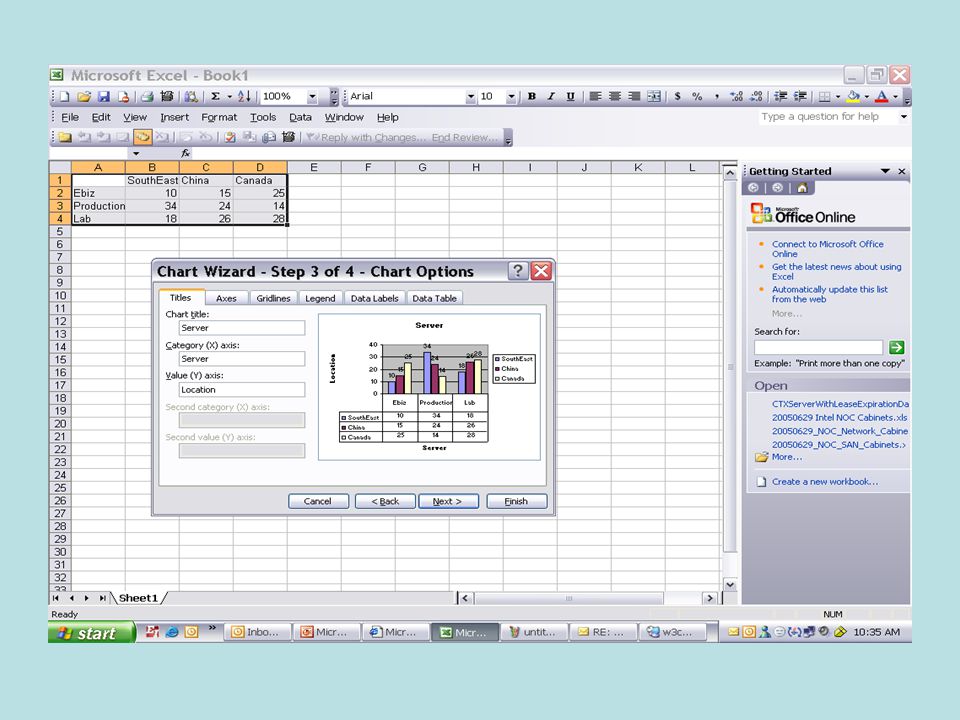
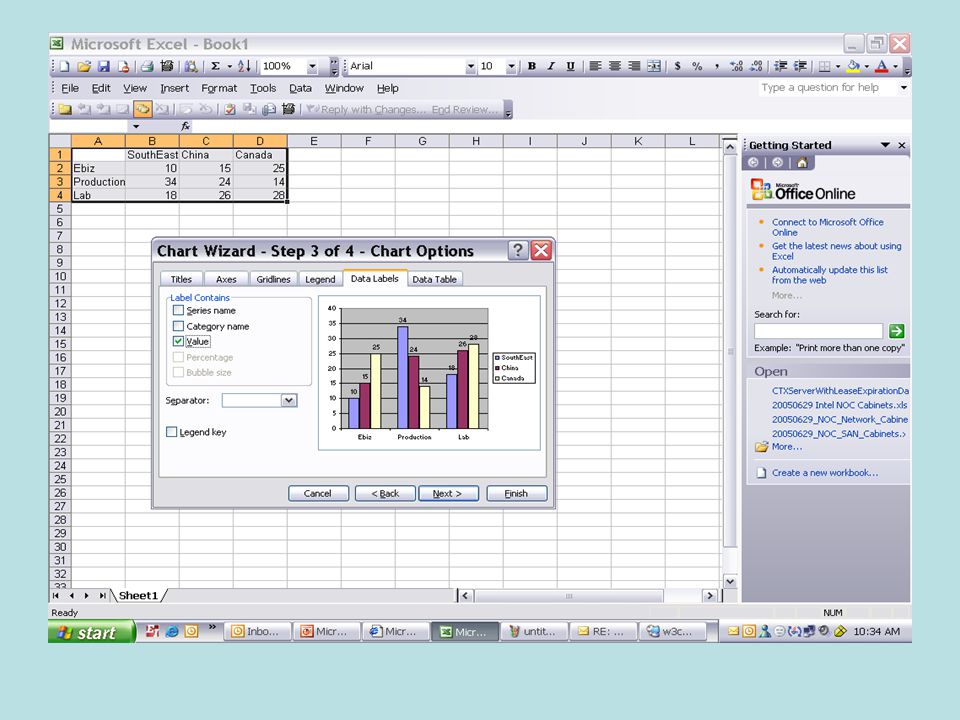
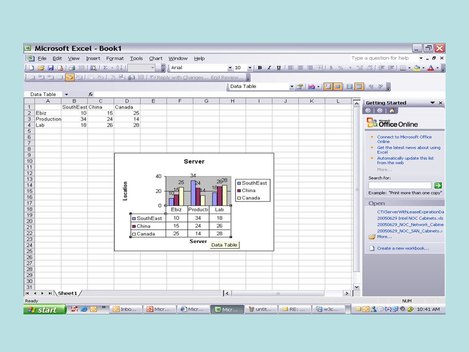
Click Next. To place the product names on the x-axis, select the Columns radio button. Type Server in the Chart Title field. Server will appear as the title of your chart. Type Server in the Category (X) Axis field. Products will appear as your x-axis title. Type Location in the Value (Y) Axis field. Location will appear as your y-axis title. Choose the Data Labels tab. Select Value in the Labels Contain Frame to display the data labels as values. Choose the Data Table tab. Select Show Data Table. The data table will appear below your chart. Choose As Object In Sheet1 to make your chart an embedded object and part of the worksheet. Click Finish Your chart will appear on the spreadsheet
 Axis field. Products will appear as your x-axis title. Type Location in the Value (Y) Axis field. Location will appear as your y-axis title. Choose the Data Labels tab. Select Value in the Labels Contain Frame to display the data labels as values. Choose the Data Table tab. Select Show Data Table. The data table will appear below your chart. Choose As Object In Sheet1 to make your chart an embedded object and part of the worksheet. Click Finish. Your chart will appear on the spreadsheet.")
73
Exercises

Similar presentations


. Is a spreadsheet application designed to take advantage of the windows graphical interface MICROSOFT EXCEL.>")


 Excel Lessons 4 – 8 Press space bar to Advance Frame.>")


 OR Click on Start All Programs Microsoft Office Microsoft Office Excel 2003.>")


