2. Outline Abstract Introduction Methodology Results

3. Abstract interpolatedcontinuous-valued heart rate signals Most of the currently accepted approaches to compute heart rate and assess heart rate variability operate on interpolated, continuous-valued heart rate signals, thereby ignoring the underlying discrete structure of human heart beats. To overcome this limitation, we model the stochastic structure of heart beat intervals as a history-dependent, inverse Gaussian process and derive from it an explicit probability density describing heart rate and heart rate variability.

4. We estimate the parameters of the inverse Gaussian model by local maximum likelihood and assess model goodness-of-fit using Q-Q plot analyses (Quantile-Quantile Normal Plots- 常態分位數圖 ) goodness-of-fit ( 適合度 ): 此種檢定是看我們之實際值 ( 或觀測值 ) 是否服從某一理 論之分配。這種實際值（或觀測值）與理論值之間之配 合程度之檢定問題稱之為適合度檢定。

5. We apply our model in an analysis of human heart beat intervals from a tilt-table experiment.

6. Introduction In the last 40 years, heart rate (HR) and heart rate variability (HRV) have been established as important quantitative indices of cardiovascular control by the autonomic nervous system, as well as effective diagnostic tools and predictors of mortality for diseases related to cardiovascular function and regulation

7. HR is the number of R-wave events (heart beats) per unit time on the electrocardiogram (ECG). HRV is defined as the variation in the R-R intervals, i.e., in the times between the R-wave events. Neither HR nor HRV can be observed directly from the ECG, but both must be estimated from the sequence of R-R intervals

8. There are several methodological limitations to current methods used to estimate HRV. In research studies, current time domain, frequency domain, dynamical systems, and entropy methods for HRV analysis generally require several minutes or more of ECG measurements in order to produce meaningful analyses, and these data often must be collected under stationary conditions.

9. In addition, most of these methods must convert R-R interval data into evenly spaced, continuous-valued measurements for analysis by first interpolating the HR series estimate computed from either the local averages model or the reciprocal model While all of these methods give important characterizations of human heart beat dynamics, none provides a goodness-of-fit assessment to measure how well the R-R interval data are described by a particular model.

10. In response to these shortcomings, we present a new statistical framework that models the R-wave events as a discrete event defined by an inverse Gaussian parametric probability function As such, our approach is able to avoid the need for conversion to continuous-valued signals and is also able to formally assess model goodness-of-fit through well established techniques for comparing discrete events models.

11. Methdology A. Heart Rate Probability Model In an observation interval (0,T] 0 <U 1 <U 2 <...,<U 5..., <U n ≦ T as the N successive R- wave event times detected from an ECG. H u n is the history of the R-R intervals up to U n θ is a set of p model parameters

12. The history term represents the influence of recent parasympathetic and sympathetic inputs to the SA node on the R-R interval length by modeling the mean as a linear function of the previous R-R intervals. The Mean and Standard deviation of the R-R interval probability model in (1) are, respectively:

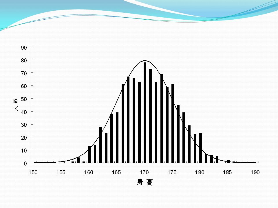
13. 高斯分佈 早在 18 世紀就有數學家和天文學家開始探討這樣的一 條曲線。德國天文家兼數學家高斯（ Carl Friedrich Gauss ， 1777-1855 ）利用常態分佈研究天文學觀察 中誤差的分佈情形，因此常態分佈又稱高斯分佈。 另一位著名的數學和統計學家 Karl Pearson （ 1857- 1936 ）將高斯分佈稱為常態分佈。

15. 這條曲線的數學函數為 其中 p = 3.1416 ， e 是自然對數之底 2.7183 ， X 介在正 負無限大， m 是平均數， s 是標準差。一旦確定平均數 和標準差後，帶入公式算得 f(X) 。

16. 要決定常態分佈的形狀，就必須知道平均數 m 和變異數 s 2 （或者標準差 s ）。常態分佈取決於兩個參數 （ parameter ）： m 和 s 2 。 只要設定這兩個參數，就可以畫出那條常態分佈曲線。只 要 m 或 s 2 不同，曲線就不同。 這也就是為何在上述公式裡，表明 其中分號後面代表的就 是決定這個函數的參數。假如變數 X 服從常態分佈，平均 數為 m ，變異數為 s 2 ，則寫成： X ~ N(m, s 2 ) ，其中 ~ 表示 服從， N 表示常態分佈。

19. B. Model Goodness-of-Fit Because the R-R interval model in (1) defines an explicit discrete event model, we can use a quantile- quantile (Q-Q) analysis to evaluate model goodness- of-fit

21. Result

22. Fig. 2. Autoregressive spectral estimation of the supine (top panel) and the tilt (bottom panel) segments of the interpolated reciprocal R-R intervals in Fig. 1A (dotted line) and our HR estimates in Fig. 1C (solid line).