1. Copyright © 2015 John, Wiley & Sons, Inc. All rights reserved. W ALTER E NDERS, U NIVERSITY OF A LABAMA A PPLIED E CONOMETRIC T IME S ERIES 4 TH ED. W ALTER E NDERS

2. Copyright © 2015 John, Wiley & Sons, Inc. All rights reserved.

3. The Random Walk Model y t = y t–1 +  t (or  y t  t ). Given the first t realizations of the {  t } process, the conditional mean of y t+1 is E t y t+1 = E t (y t +  t+1 ) = y t Similarly, the conditional mean of y t+s (for any s > 0) can be obtained from Hence var(y t ) = var(  t +  t–1 +... +  1 ) = t  2 var(y t–s ) = var(  t–s +  t–s–1 +... +  1 ) = (t – s 

4. Copyright © 2015 John, Wiley & Sons, Inc. All rights reserved. Random Walk Plus Drift y t = y t–1 + a 0 +  t Given the initial condition y 0, the general solution for y t is E t y t+s = y t + a 0 s.

5. Copyright © 2015 John, Wiley & Sons, Inc. All rights reserved. E[(y t – y 0 )(y t–s – y 0 )] = E[(  t +  t–1 +...+  1 )(  t–s +  t–s–1 +...+  1 )] = E[(  t–s ) 2 +(  t–s–1 ) 2 +...+(  1 ) 2 ] = (t – s)  2 The autocorrelation coefficient = [(t – s)/t] 0.5 Hence, in using sample data, the autocorrelation function for a random walk process will show a slight tendency to decay.

6. Copyright © 2015 John, Wiley & Sons, Inc. All rights reserved.

8. Table 4.1: Selected Autocorrelations From Nelson and Plosser

9. Copyright © 2015 John, Wiley & Sons, Inc. All rights reserved. Worksheet 4.1

10. Copyright © 2015 John, Wiley & Sons, Inc. All rights reserved. Consider the two random walk plus drift processes y t = 0.2 + y t  1 +  yt z t =  0.1 + z t  1 +  zt Here {y t } and {z t } series are unit-root processes with uncorrelated error terms so that the regression is spurious. Although it is the deterministic drift terms that cause the sustained increase in y t and the overall decline in z t, it appears that the two series are inversely related to each other. The residuals from the regression y t = 6.38  0.10z t are nonstationary. Scatter Plot of y t Against z t Regression Residuals Worksheet 4.2

11. Copyright © 2015 John, Wiley & Sons, Inc. All rights reserved.

12. 3. UNIT ROOTS AND REGRESSION RESIDUALS y t = a 0 + a 1 z t + e t Assumptions of the classical model: – both the {y t } and {z t } sequences be stationary – the errors have a zero mean and a finite variance. – In the presence of nonstationary variables, there might be what Granger and Newbold (1974) call a spurious regression A spurious regression has a high R 2 and t-statistics that appear to be significant, but the results are without any economic meaning. The regression output “looks good” because the least- squares estimates are not consistent and the customary tests of statistical inference do not hold.

13. Copyright © 2015 John, Wiley & Sons, Inc. All rights reserved. Four cases CASE 1: Both {y t } and {z t } are stationary. – the classical regression model is appropriate. CASE 2: The {y t } and {z t } sequences are integrated of different orders. – Regression equations using such variables are meaningless CASE 3: The nonstationary {y t } and {z t } sequences are integrated of the same order and the residual sequence contains a stochastic trend. – This is the case in which the regression is spurious. – In this case, it is often recommended that the regression equation be estimated in first differences. CASE 4: The nonstationary {y t } and {z t } sequences are integrated of the same order and the residual sequence is stationary. – In this circumstance, {y t } and {z t } are cointegrated.

14. Copyright © 2015 John, Wiley & Sons, Inc. All rights reserved. The Dickey-Fuller tests The  1,  2, and  3 statistics are constructed in exactly the same way as ordinary F-tests:

15. Copyright © 2015 John, Wiley & Sons, Inc. All rights reserved.

16. Table 4.2: Summary of the Dickey-Fuller Tests

17. Copyright © 2015 John, Wiley & Sons, Inc. All rights reserved. Table 4.3: Nelson and Plosser's Tests For Unit Roots p is the chosen lag length. Entries in parentheses represent the t-test for the null hypothesis that a coefficient is equal to zero. Under the null of nonstationarity, it is necessary to use the Dickey-Fuller critical values. At the.05 significance level, the critical value for the t-statistic is -3.45.

18. Copyright © 2015 John, Wiley & Sons, Inc. All rights reserved. Quarterly Real U.S. GDP  lrgdp t = 0.1248 + 0.0001t  0.0156lrgdp t–1 + 0.3663  lrgdp t–1 (1.58) (1.31) (  1.49) (6.26) The t-statistic on the coefficient for lrgdp t–1 is  1.49. Table A indicates that, with 244 usable observations, the 10% and 5% critical value of   are about  3.13 and  3.43, respectively. As such, we cannot reject the null hypothesis of a unit root. The sample value of  3 for the null hypothesis a 2 =  = 0 is 2.97. As Table B indicates that the 10% critical value is 5.39, we cannot reject the joint hypothesis of a unit root and no deterministic time trend. The sample value of  2 is 20.20. Since the sample value of  2 (equal to 17.61) far exceeds the 5% critical value of 4.75, we do not want to exclude the drift term. We can conclude that the growth rate of the real GDP series acts as a random walk plus drift plus the irregular term 0.3663  lrgdp t–1.

19. Copyright © 2015 John, Wiley & Sons, Inc. All rights reserved. Table 4.4: Real Exchange Rate Estimation  H 0 :  = 0 LagsMean  / DW F SD/ SEE 1973-1986 Canada  0.022 (0.016) t =  1.42 01.05 0.059 1.88 0.194 5.47 1.16 Japan  0.047 (0.074) t =  0.64 21.01  0.007 2.01 0.226 10.44 2.81 Germany  0.027 (0.076) t =  0.28 21.11  0.014 2.04 0.858 20.68 3.71 1960-1971 Canada  0.031 (0.019) t =  1.59 01.02  0.107 2.21 0.434.014.004 Japan  0.030 (0.028) t =  1.04 00.98 0.046 1.98 0.330.017.005 Germany  0.016 (0.012) t =  1.23 01.010.038 1.93 0.097.026.004

20. Copyright © 2015 John, Wiley & Sons, Inc. All rights reserved. EXTENSIONS OF THE DICKEY–FULLER TEST y t = a 0 + a 1 y t–1 + a 2 y t–2 + a 3 y t–3 +... + a p–2 y t–p+2 + a p–1 y t–p+1 + a p y t–p +  t add and subtract a p y t–p+1 to obtain y t = a 0 + a 1 y t–1 + a 2 y t–2 +...+ a p–2 y t–p+2 + (a p–1 + a p )y t–p+1 – a p  y t–p+1 +  t Next, add and subtract (a p–1 + a p )y t–p+2 to obtain: y t = a 0 + a 1 y t–1 + a 2 y t–2 + a 3 y t–3 +... – (a p–1 + a p )  y t–p+2 – a p  y t–p+1 +  t Continuing in this fashion, we obtain

21. Copyright © 2015 John, Wiley & Sons, Inc. All rights reserved. Rule 1: Consider a regression equation containing a mixture of I(1) and I(0) variables such that the residuals are white noise. If the model is such that the coefficient of interest can be written as a coefficient on zero-mean stationary variables, then asymptotically, the OLS estimator converges to a normal distribution. As such, a t-test is appropriate.

22. Copyright © 2015 John, Wiley & Sons, Inc. All rights reserved. Rule 1 indicates that you can conduct lag length tests using t- tests and/or F-tests on  y t =  y t–1 +  2  y t–1 +  3  y t–2 + … +  p  y t–p+1 +  t

23. Copyright © 2015 John, Wiley & Sons, Inc. All rights reserved. Selection of the Lag Length general-to-specific methodology – Start using a lag length of p*. If the t-statistic on lag p* is insignificant at some specified critical value, re- estimate the regression using a lag length of p*–1. Repeat the process until the last lag is significantly different from zero. – Once a tentative lag length has been determined, diagnostic checking should be conducted. Model Selection Criteria (AIC,SBC) Residual-based LM tests

24. Copyright © 2015 John, Wiley & Sons, Inc. All rights reserved. The Test with MA Components A(L)y t = C(L)  t so that A(L)/C(L)y t =  t So that D(L)y t =  t – Even though D(L) will generally be an infinite- order polynomialwe can use the same technique as used above to form the infinite-order autoregressive model – However, unit root tests generally work poorly if the error process has a strongly negative MA component.

25. Copyright © 2015 John, Wiley & Sons, Inc. All rights reserved. Example of a Negative MA term y t = y t-1 + ε t – β 1 ε t-1 ; 0 < β 1 < 1. The ACF is: γ 0 = E[(y t – y 0 ) 2 ] = σ 2 + (1 – β 1 ) 2 E[(ε t-1 ) 2 + (ε t-2 ) 2 + … + (ε 1 ) 2 ] = [1 + (1 – β 1 ) 2 (t – 1)]σ 2 γ s = E[(y t – y 0 )(y t-s – y 0 )] = E[(ε t +(1–β 1 )ε t-1 + … + (1–β 1 )ε 1 )(ε t-s + (1–β 1 )ε t-s-1 + … + (1–β 1 )ε 1 ) = (1 – β 1 ) [1 + (1 – β 1 ) (t – s – 1)] σ 2 The ρ i approach unity as the sample size t becomes infinitely large. For the sample sizes usually found in applied work, the autocorrelations can be small. Let β 1 be close to unity so that terms containing (1 – β 1 ) 2 can be safely ignored. The ACF can be approximated by ρ 1 = ρ 2 = … = (1 – β 1 ) 0.5. For example, if β 1 = 0.95, all of the autocorrelations should be 0.22.

26. Copyright © 2015 John, Wiley & Sons, Inc. All rights reserved. Multiple Roots Consider  2 y t = a 0 +  1  y t–1 +  t If  1 does differ from zero, estimate  2 y t = a 0 +  1  y t–1 +  2 y t–1 +  t If you reject the null hypothesis,  2 = 0,conclude that {y t } is stationary.

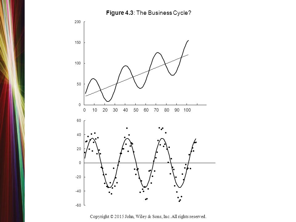
27. Copyright © 2015 John, Wiley & Sons, Inc. All rights reserved. Panel (a) y t = 0.5y t−1 +  t + D L Panel (b) y t = y t−1 +  t + D P Figure 4.9 Two Models of Structural Change

28. Copyright © 2015 John, Wiley & Sons, Inc. All rights reserved. Perron’s Test Let the null be y t = a 0 + y t–1 +  1 D P +  2 D L +  t – where D P and D L are the pulse and level dummies Estimate the regression (the alternative): y t = a 0 + a 2 t +m 1 D P + m 2 D L + m 3 D T +  t – Let D T be a trend shift dummy such that D T = t –  for t >  and zero otherwise. Now consider a regression of the residuals If the errors do not appear to be white noise, estimate the equation in the form of an augmented Dickey–Fuller test. The t-statistic for the null hypothesis a 1 = 1 can be compared to the critical values calculated by Perron (1989). For = 0.5, Perron reports the critical value of the t-statistic at the 5 percent significance level to be –3.96 for H 2 and –4.24 for H 3.

29. Copyright © 2015 John, Wiley & Sons, Inc. All rights reserved. Table 4.6: Retesting Nelson and Plosser's Data For Structural Change The appropriate t-statistics are in parenthesis. For a 0,  1,  2, and a 2, the null is that the coefficient is equal to zero. For a 1, the null hypothesis is a 1 = 1. Note that all estimated values of a 1 are significantly different from unity at the 1% level. T k a 0  1  2 a 2 a 1 Real GNP620.338 3.44 (5.07) -0.189 (-4.28) -0.018 (-0.30) 0.027 (5.05) 0.282 (-5.03) Nominal GNP 620.338 5.69 (5.44) -3.60 (-4.77) 0.100 (1.09) 0.036 (5.44) 0.471 (-5.42) Industrial Prod. 1110.6680.120 (4.37) -0.298 (-4.56) -0.095 (-.095) 0.032 (5.42) 0.322 (-5.47)

30. Copyright © 2015 John, Wiley & Sons, Inc. All rights reserved. Power Formally, the power of a test is equal to the probability of rejecting a false null hypothesis (i.e., one minus the probability of a type II error). The power for tau-mu is

31. Copyright © 2015 John, Wiley & Sons, Inc. All rights reserved. Nonlinear Unit Root Tests Enders-Granger Test  y t = I t  1 (y t–1 –  ) + (1 – I t )  2 (y t–1 –  ) +  t LSTAR and ESTAR Tests Nonlinear Breaks—Endogenous Breaks

32. Copyright © 2015 John, Wiley & Sons, Inc. All rights reserved. Schmidt and Phillips (1992) LM Test The overly-wide confidence intervals for  means that you are less likely to reject the null hypothesis of a unit root even when the true value of  is not zero. A number of authors have devised clever methods to improve the estimates of the intercept and trend coefficients.  y t = a 2 +  t The idea is to estimate the trend coefficient, a 2, using the regression  y t = a 2 +  t. As such, the presence of the stochastic trend  i does not interfere with the estimation of a 2.

33. Copyright © 2015 John, Wiley & Sons, Inc. All rights reserved. LM Test Continued Use this estimate to form the detrended series as Then use the detrended series to estimate Schmidt and Phillips (1992) show that it is preferable to estimate the parameters of the trend using a model without the persistent variable y t-1. Elliott, Rothenberg and Stock (1996) show that it is possible to further enhance the power of the test by estimating the model using something close to first-differences.

34. Copyright © 2015 John, Wiley & Sons, Inc. All rights reserved. The Elliott, Rothenberg, and Stock Test Instead of creating the first difference of y t, Elliott, Rothenberg and Stock (ERS) preselect a constant close to unity, say , and subtract  y t  1 from y t to obtain: = a 0 + a 2 t   a 0   a 2 (t  1) + e t, for t = 2, …, = (1   )a 0 + a 2 [(1  )t +  )] + e t. = a 0 z1 t + a 2 z2 t + e t z1 t = (1   ) ; z2 t =  + (1  )t. The important point is that the estimates a 0 and a 2 can be used to detrend the {y t } series

35. Copyright © 2015 John, Wiley & Sons, Inc. All rights reserved. Panel Unit Root Tests  y it = a i0 +  i y it–1 + a i2 t + +  it One way to obtain a more powerful test is to pool the estimates from a number separate series and then test the pooled value. The theory underlying the test is very simple: if you have n independent and unbiased estimates of a parameter, the mean of the estimates is also unbiased. More importantly, so long as the estimates are independent, the central limit theory suggests that the sample mean will be normally distributed around the true mean. – The difficult issue is to correct for cross equation correlation Because the lag lengths can differ across equations, you should perform separate lag length tests for each equation. Moreover, you may choose to exclude the deterministic time trend. However, if the trend is included in one equation, it should be included in all

36. Copyright © 2015 John, Wiley & Sons, Inc. All rights reserved. Lags Estimated  i t-statistic Estimated  i t-statistic Log of the Real RateMinus the Common Time Effect Australia5-0.049-1.678 -0.043-1.434 Canada7-0.036-1.896 -0.035-1.820 France1-0.079-2.999 -0.102-3.433 Germany1-0.068-2.669 -0.067-2.669 Japan3-0.054-2.277 -0.048-2.137 Netherlands1-0.110-3.473 -0.137-3.953 U.K.1-0.081-2.759 -0.069-2.504 U.S.1-0.037-1.764 -0.045-2.008 Table 4.8: The Panel Unit Root Tests for Real Exchange Rates

37. Copyright © 2015 John, Wiley & Sons, Inc. All rights reserved. Limitations The null hypothesis for the IPS test is  i =  2 = … =  n = 0. Rejection of the null hypothesis means that at least one of the  i ’s differs from zero. At this point, there is substantial disagreement about the asymptotic theory underlying the test. Sample size can approach infinity by increasing n for a given T, increasing T for a given n, or by simultaneously increasing n and T. – For small T and large n, the critical values are dependent on the magnitudes of the various  ij. The test requires that that the error terms be serially uncorrelated and contemporaneously uncorrelated. – You can determine the values of p i to ensure that the autocorrelations of {  it } are zero. Nevertheless, the errors may be contemporaneously correlated in that E  it  jt  0 – The example above illustrates a common technique to correct for correlation across equations. As in the example, you can subtract a common time effect from each observation. However, there is no assurance that this correction will completely eliminate the correlation. Moreover, it is quite possible that is nonstationary. Subtracting a nonstationary component from each sequence is clearly at odds with the notion that the variables are stationary.

38. Copyright © 2015 John, Wiley & Sons, Inc. All rights reserved. The Beveridge-Nelson Decomposition The trend is defined to be the conditional expectation of the limiting value of the forecast function. In lay terms, the trend is the “long-term” forecast. This forecast will differ at each period t as additional realizations of {e t } become available. At any period t, the stationary component of the series is the difference between y t and the trend  t.

39. Copyright © 2015 John, Wiley & Sons, Inc. All rights reserved. BN 2 Estimate the {y t } series using the Box–Jenkins technique. – After differencing the data, an appropriately identified and estimated ARMA model will yield high-quality estimates of the coefficients. Obtain the one-step-ahead forecast errors of E t y t+s for large s. Repeating for each value of t yields the entire set of premanent components The irregular component is y t minus the value of the trend.

40. Copyright © 2015 John, Wiley & Sons, Inc. All rights reserved. The HP Filter For a given value of  the goal is to select the {  t } sequence so as to minimize this sum of squares. In the minimization problem is an arbitrary constant reflecting the “cost” or penalty of incorporating fluctuations into the trend. In applications with quarterly data, including Hodrick and Prescott (1984) is usually set equal to 1,600. Large values of acts to “smooth out” the trend. Let the trend of a nonstationary series be the {  t } sequence so that y t –  t the stationary component

41. Copyright © 2015 John, Wiley & Sons, Inc. All rights reserved.