1. Note – throughout figures the boundary layer thickness is greatly exaggerated! CHAPTER 9: EXTERNAL INCOMPRESSIBLE VISCOUS FLOWS Can’t have fully developed flow Velocity profile evolves, flow is accelerating Generally boundary layers (Re x > 10 4 ) are very thin.

2. Laminar Flow  /x ~ 5.0/Re x 1/2 THEORY Turbulent Flow (Re x > 10 6 )  /x ~ 0.16/Re x 1/7 EXPERIMENTAL “At these Re x numbers bdy layers so thin that displacement effect on outer inviscid layer is small”

4. Blasius showed theoretically that  /x = 5/Re x (Re x =  U  x/  ) BOUNDARY LAYER THICKNESS:  is y where u(x,y) = 0.99 U  This definition for  is completely arbitrary, why not 98%, 95%, etc.

5. Because of the velocity deficit, U-u, within the bdy layer, the mass flux through b-b is less than a-a. However if we displace the plate a distance  *, the mass flux along each section will be identical. DISPLACEMENT THICKNESS:  * = 0   (1 – u/U)dy

6. u U [(u)(  [U-u])] [Flux of momentum deficit]  U 2  = total flux of momentum deficit The momentum thickness, , is defined as the thickness of a layer of fluid, with velocity U e, for which the momentum flux is equal to the deficit of momentum flux through the boundary layer.  U e 2  = 0    u(U e – u)dy  = 0   [u/U e ] (1 – u/U e )dy

7. Want to relate momentum thickness, , with drag, D, on plate U e is constant so  p/  dx = 0; Re < 100,000 so laminar, flow is steady,  is small (so  * is small) so  p/  y ~ 0 Conservation of Mass: -  U e hw +  0 h uwdy +  0 L vwdx = 0 Ignoring the fact that because of  *, U e is not parallel to plate Jason Batin, what are forces on control volume?

8. X-component of Momentum Equation  p/  dx = 0  p/  dy = 0  U e /  y = 0 -D = -  U e 2 hw +  0 h u 2 wdy +  0 L U e vwdx v is bringing U e out of control volume a-b c-d b-c

9. X-component of Momentum Equation  p/  dx = 0  U e /  y = 0 -D = -  U e 2 hw +  0 h u 2 wdy +  0 L U e vwdx Conservation of Mass: -  U e hw +  0 h uwdy +  0 L vwdx = 0 -  U e 2 hw +  0 h uU e wdy +  0 L vU e wdx = 0

10. X-component of Momentum Equation  p/  dx = 0  U e /  y = 0 -D = -  U e 2 hw+  0 h u 2 wdy +  U e 2 hw-  0 h uU e wdy -D =  0 h u 2 wdy +  0 h uU e wdy D/(  U e 2 w) =  0 h (-u 2 /U e 2 ) dy +  0 h (u/U e )wdy D/(  U e 2 w) =  0 h (u/U e )[1-u/U e ] dy ~  0  (u/U e )[1-u/U e ] dy = 

11.  p/  dx = 0  U e /  y = 0 D/(  U e 2 w) =  D =  U e 2 w  dD/dx =  U e 2 w(d  /dx) D =  0 L  wall wdx (all skin friction) dD/dx =  wall w =  U e 2 w(d  /dx)

12.  p/  dx = 0  U e /  y = 0 D =  U e 2 w  dD/dx =  wall w =  U e 2 w(d  /dx) knowing u(x,y) then can calculate  and from  can calculate drag and  wall the change in drag along x occurs at the expense on an increase in  which represents a decrease in the momentum of the fluid

13. SIMPLIFYING ASSUMPTIONS OFTEN MADE FOR ENGINERING ANALYSIS OF BOUNDARY LAYER FLOWS

14. Blasius developed an exact solution (but numerical integration was necessary) for laminar flow with no pressure variation. Blasius could theoretically predict: boundary layer thickness  (x), velocity profile u(x,y)/U  Moreover: u(x,y)/U  vs y/  is self similar and wall shear stress  w (x).

15. Dimensionless velocity profile for a laminar boundary layer: comparison with experiments by Liepmann, NACA Rept. 890, 1943. Adapted from F.M. White, Viscous Flow, McGraw-Hill, 1991

16. Blasius developed an exact solution (but numerical integration was necessary) for laminar flow with no pressure variation. Blasius could theoretically predict boundary layer thickness  (x), velocity profile u(x,y)/U  vs y/ , and wall shear stress  w (x). Von Karman and Poulhausen derived momentum integral equation (approximation) which can be used for both laminar (with and without pressure gradient) and turbulent flow

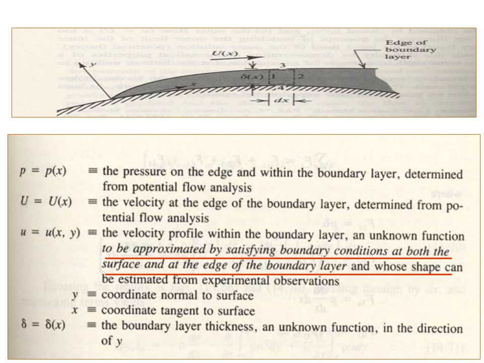
17. Von Karman and Polhausen method (MOMENTUM INTEGRAL EQ. Section 9-4) devised a simplified method by satisfying only the boundary conditions of the boundary layer flow rather than satisfying Prandtl’s differential equations for each and every particle within the boundary layer.

19. WHERE WE WANT TO GET…

20. Deriving MOMENTUM INTEGLAL EQ so can calculate  (x),  w.

21. u(x,y) Surface Mass Flux Through Side ab

22. Surface Mass Flux Through Side cd

23. Surface Mass Flux Through Side bc

24. Assumption : (1) steady (3) no body forces Apply x-component of momentum eq. to differential control volume abcd u

25. mf represents x-component of momentum flux; F sx will be composed of shear force on boundary and pressure forces on other sides of c.v.

26. X-momentum Flux =  cv u  V  dA Surface Momentum Flux Through Side ab u

27. X-momentum Flux =  cv u  V  dA Surface Momentum Flux Through Side cd u

28. U=U e =U  X-momentum Flux =  cv u  V  dA Surface Momentum Flux Through Side bc u

29. a-bc-d b-c X-Momentum Flux Through Control Surface

30. IN SUMMARY RHS X-Momentum Equation

31. X-Force on Control Surface w is unit width into page p(x) Surface x-Force On Side ab Note that p  f(y) w

32. w is unit width into page p(x+dx) Surface x-Force On Side cd

33. Surface x-Force On Side bc p + ½ [dp/dx]dx is average pressure along bc Force in x-direction: [p + ½ (dp/dx)] wd  w

34. Why  and not (bc)? w

35. Surface x-Force On Side bc   psin  in x-direction; (A)(psin  ) is force in x-direction Asin  =  w So force in x-direction = p  w  psin  w A p

36. Note that since the velocity gradient goes to zero at the top of the boundary layer, then viscous shears go to zero. Surface x-Force On Side bc

37. -(  w + ½ d  w /dx] x dx)wdx Surface x-Force On Side ad

38. F x = F ab + F cd + F bc + F ad F x = pw  -(p + [dp/dx] x dx) w(  + d  ) + (p + ½ [dp/dx] x dx)wd  - (  w + ½ (d  w /dx)  x dx)wdx F x = pw  -(p w  + p wd  + [dp/dx] x dx) w  + [dp/dx] x dx w d  ) + (p wd  + ½ [dp/dx] x dxwd  ) - (  w + ½ (d  w /dx)  x dx)wdx d  <<  = - ½ (d  w /dx  x dx)dx d  w <<  w p(x) **+ + # #

39. =

40. ab -cdbc U

41. Divide by wdx dp/dx = -  UdU/dx for inviscid flow outside bdy layer  =  from 0 to  of dy

42. Integration by parts Multiply by U 2 /U 2 Multiply by U/U

46. If flow at B did not equal flow at C then could connect and make perpetual motion machine. C C

48. HARDEST PROBLEM – WORTH NO POINTS …BUT MAYBE PEACE OF MIND

50. (plate is 2% thick, Re x=L = 10,000; air bubbles in water) For flat plate with dP/dx = 0, dU/dx = 0

51. Realize (like Blasius) that u/U similar for all x when plotted as a function of y/ . Substitutions:  = y/  ; so dy =  d   = y/   =0 when y=0  =1 when y=  u/U  ~ y/ 

53.  = 0  u/U e (1 – u/U e )dy  = y/  ; d  = dy/  Strategy: obtain an expression for  w as a function of , and solve for  (x)  (0.133 for Blasius exact solution, laminar, dp/dx = 0)

54. Laminar Flow Over a Flat Plate, dp/dx = 0 Assume velocity profile: u = a + by + cy 2 B.C. at y = 0u = 0so a = 0 at y =  u = Uso U = b  + c  2 at y =   u/  y = 0 so 0 = b + 2c  and b = -2c  U = -2c  2 + c  2 = -c  2 so c = -U/  2 u = -2c  y – (U/  2 ) y 2 = 2U  y/  2 – (U/  2 ) y 2 u/U = 2(y/  ) – (y/  ) 2 Let y/  =  u/U = 2  -  2 Want to know  w (x) Strategy: obtain an expression for  w as a function of , and solve for  (x)

55. Laminar Flow Over a Flat Plate, dp/dx = 0 u/U = 2  -  2 Strategy: obtain an expression for  w as a function of , and solve for  (x)

56. u/U = 2  -  2 2  - 4  2 + 2  3 -  2 +2  3 -  4 Strategy: obtain an expression for  w as a function of , and solve for  (x)

57. 2  U/(  U 2 ) = (d  /dx) (  2 – (5/3)  3 +  4 – (1/5)  5 )| 0 1 2  U/(  U 2 ) = (d  /dx) (1 – 5/3 + 1 – 1/5) = (d  /dx) (2/15) Assuming  = 0 at x = 0, then c = 0  2 /2 = 15  x/(  U) Strategy: obtain an expression for  w as a function of , and solve for  (x)

58.  2 /2 = 15  x/(  U)  2 /x 2 = 30  /(  Ux) = 30 Re x  /x = 5.5 (Re x ) -1/2   x 1/2 Strategy: obtain an expression for  w as a function of , and solve for  (x)

59. THE END

60. Illustration of strong interaction between viscid and inviscid regions in the rear of a blunt body. Re = 15,000 Re = 17.9 (separation at Re = 24)

61. Re = 20,000 Angle of attack = 6 o Symmetric Airfoil 16% thick

62. Laminar Flow Over a Flat Plate, dp/dx = 0 Assume velocity profile: u = a + by + cy 2 B.C. at y = 0u = 0so a = 0 at y =  u = Uso U = b  + c  2 at y =   u/  y = 0 so 0 = b + 2c  and b = -2c  U = -2c  2 + c  2 = -c  2 so c = -U/  2 u = -2c  y – (U/  2 ) y 2 = 2U  y/  2 – (U/  2 ) y 2 u/U = 2(y/  ) – (y/  ) 2 Let y/  =  u/U = 2  -  2 