2. Quanitification of BL Effects in Engineering Utilitites… P M V Subbarao Professor Mechanical Engineering Department I I T Delhi Engineering Parameters for Flat Plate Boundary Layer Solutions

3. ODE for Flat Plate Boundary Layer

4. 3 BL ODE

5. The Blasius Equation The Blasius equation with the above boundary conditions exhibits a boundary value problem. However, one boundary is unknown, though boundary condition is known. However, using an iterative method, it can be converted into an initial value problem. Assuming a certain initial value for F  =0 , Blasius equation can be solved using Runge-Kutta or Predictor- Corrector methods

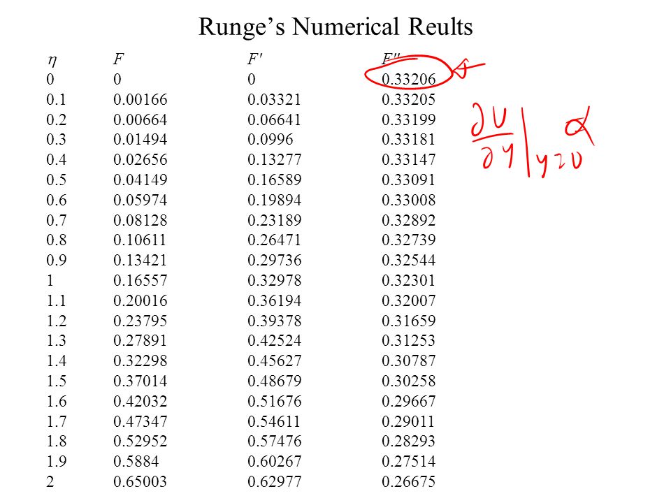
7.  FF'F'' 0000.33206 0.10.001660.033210.33205 0.20.006640.066410.33199 0.30.014940.09960.33181 0.40.026560.132770.33147 0.50.041490.165890.33091 0.60.059740.198940.33008 0.70.081280.231890.32892 0.80.106110.264710.32739 0.90.134210.297360.32544 10.165570.329780.32301 1.10.200160.361940.32007 1.20.237950.393780.31659 1.30.278910.425240.31253 1.40.322980.456270.30787 1.50.370140.486790.30258 1.60.420320.516760.29667 1.70.473470.546110.29011 1.80.529520.574760.28293 1.90.58840.602670.27514 2 0.650030.629770.26675 Runge’s Numerical Reults

8. 2.20.78120.681320.24835 2.30.850560.705660.23843 2.40.92230.728990.22809 2.50.996320.751270.21741 2.61.072510.772460.20646 2.71.150770.792550.19529 2.81.230990.811520.18401 2.91.313040.829350.17267 31.396820.846050.16136 3.11.482210.861620.15016 3.21.569110.876090.13913 3.31.657390.889460.12835 3.41.746960.901770.11788 3.51.837710.913050.10777 3.61.929540.923340.09809 3.72.022350.932680.08886 3.82.116040.941120.08013 3.92.210540.948720.07191  FF'F''

9. 42.305760.955520.06423 4.12.401620.961590.0571 4.22.498060.966960.05052 4.32.5950.971710.04448 4.42.692380.975880.03897 4.52.790150.979520.03398 4.62.888270.982690.02948 4.72.986680.985430.02546 4.83.085340.987790.02187 4.93.184220.989820.0187 53.28330.991550.01591 5.13.382530.993010.01347 5.23.481890.994250.01134 5.33.581370.995290.00951 5.43.680940.996160.00793 5.53.78060.996880.00658  FF'F''

10. 5.63.880320.997480.00543 5.73.980090.997980.00446 5.84.079910.998380.00365 5.94.179760.998710.00297 64.279650.998980.0024 6.14.379560.999190.00193 6.24.479490.999370.00155 6.34.579430.999510.00124 6.44.679390.999620.00098 6.54.779350.99970.00077 6.64.879330.999770.00061 6.74.979310.999830.00048 6.85.079290.999870.00037 6.95.179280.99990.00029 75.279270.999930.00022  FF'F''

11. 7.15.379270.999950.00017 7.25.479260.999960.00013 7.35.579260.999979.8E-05 7.45.679260.999987.4E-05 7.55.779250.999995.5E-05 7.65.879250.999994.1E-05 7.75.9792513.1E-05 7.86.0792512.3E-05 7.96.1792511.7E-05 86.2792511.2E-05 8.16.3792518.9E-06 8.26.4792516.5E-06 8.36.5792514.7E-06 8.46.6792513.4E-06 8.56.7792512.4E-06 8.66.8792511.7E-06 8.76.9792511.2E-06 8.87.0792518.5E-07  FF'F''

12. 8.97.179261.000015.9E-07 97.279261.000014.1E-07 9.17.379261.000012.9E-07 9.27.479261.000012E-07 9.37.579261.000011.4E-07 9.47.679261.000019.3E-08 9.57.779261.000016.3E-08 9.67.879261.000014.3E-08 9.77.979261.000012.9E-08 9.88.079261.000011.9E-08 9.98.179261.000011.3E-08 108.279261.000018.5E-09  FF'F''

13. Recall that the nominal boundary thickness  is defined such that u = 0.99 U when y = . By interpolating on the table, it is seen that u/U = F’ = 0.99 when  = 4.91. Since u = 0.99 U when  = 4.91 and  = y[U/( x)] 1/2, it follows that the relation for nominal boundary layer thickness is NOMINAL BOUNDARY LAYER THICKNESS

14. Let the flat plate have length L and width b out of the page: DRAG FORCE ON THE FLAT PLATE L b The shear stress  o (drag force per unit area) acting on one side of the plate is given as Since the flow is assumed to be uniform out of the page, the total drag force F D acting on the plate is given as The term  u/  y =  2  /  y 2 is given from as

15. The shear stress  o (x) on the flat plate is then given as But from the table F  (0) = 0.332, so that boundary shear stress is given as Thus the boundary shear stress varies as x -1/2. A sample case is illustrated on the next slide for the case U = 10 m/s, = 1x10 -6 m 2 /s, L = 10 m and  = 1000 kg/m 3 (water).  FF'F'' 0000.33206 0.10.001660.033210.33205 0.20.006640.066410.33199 0.30.014940.09960.33181 0.40.026560.132770.33147 0.50.041490.165890.33091

16. Sample distribution of shear stress  o (x) on a flat plate: Variation of Local Shear Stress along the Length Note that  o =  at x = 0. Does this mean that the drag force F D is also infinite? U = 0.04 m/s L = 0.1 m = 1.5x10 -5 m 2 /s  = 1.2 kg/m 3 (air)

17. The drag force converges to a finite value! DRAG FORCE ON THE FLAT PLATE

18. Boundary Layer Thicknesses The application of integral balances to the control volume shown in above figure delivers more engineering properties namely, the boundary layer displacement thickness the boundary layer momentum deficiency thickness and the energy deficiency thickness.

19. Selection of a CV for Engineering BL Analysis The control volume chosen for the analysis is enclosed by dashed lines. This selection is not arbitrary but very clever. Since velocity distributions are known only at the inlet and exit, it is imperative that the other two sides on the control volume be streamlines, where no mass or momentum crosses.

20. Impermeable Streamlines of A BL The lower side should be the wall itself; hence the drag force will be exposed. The upper side should be a streamline outside the shear layer, so that the viscous drag is zero along this line.

21. The Displacement Thickness Conservation of mass is applied to this Engineering CV @SSSF: Assuming incompressible flow, this relation simplifies to

22.  * is the engineering formal definition of the boundary-layer displacement Thickness and holds true for any incompressible flow.

23. Momentum Thickness as Related to Flat-Plate Drag Conservation of Integral x momentum

24. Physical Interpretation of Momentum and displacement thicknesses Their ratio of displacement thickness to momentum thickness is called the shape factor, is often used in boundary-layer analyses:

26. Boundary layer development along a wedge We know that the velocity distribution outside the boundary layer is a simple power function

27. At the Edge of Boundary Layer

28. BL Equations for A Wedge

29. ODE for Wedge BL Flows Introducing the same relationship for the stream function as This is the so-called Falkner-Skan equation which describes a flow past a wedge.

30. Effect of Wedge Angle on BL Profile

31. Wind Tunnel Test Facility

32. Flow along a convex corner (  < 0).

33. Types of Boundary Layers If the external pressure gradient,, then, at the wall and hence is at a maximum there and falls away steadily.

34. Favourable Pressure Gradient If the external pressure gradient,, then, at the wall Must decrease faster as y increases

35. Adverse Pressure Gradient If the external pressure gradient,, then, at the wall Must Increase initially and then decrease as y increases

36. Boundary Layer Separation

37. Pressure Gradient along a cylindrical Surface