1. Frequency Response OBJECTIVE - Bode and Nyquist plots for control analysis - Determination of transfer function - Gain and Phase margins - Stability in frequency response

2. Magnitude and Phase Angle Transfer function is R(s)R(s) Y(s)Y(s) By replacing we can find its magnitude and its phase angle Higher order transfer function Can be presented in magnitude-phase form as

3. A system with transfer function of G(s) is subjected to a sinusoidal input. Determine the time response of the system. Solution The input in phasor form (magnitude-phase form) can be presented as As the transfer function is Hence the output is by replacing In time domain which give the time response of the system, the output is Example

4. First order Frequency response Its magnitude and phase angle Transfer function by replacing

5. Second order Transfer function Frequency response by replacing Its magnitude and phase angle

6. Higher Order Cascade form Frequency response by replacing Or in phasor form

7. Example: Find the frequency response of the following transfer function Example Where and

8. Respective magnitude and phase angle and Example

9. Bode Plot Consider higher order system Logarithmic form In dB. Phase angle

10. Bode Plot

11. Bode Plot for constant gain Log magnitude in dB Its phase angle >> bode([200],[1]);grid Let K=200

12. Bode Plot for constant gain

13. Bode Plot of pole on the origin Log magnitude in dB 10 10-20 10 2 -40 10 3 -60 01 10 -1 20 10 -2 40 10 -3 60

14. 10 2-6 2 -12 2323 -18 Slope of –20dB/decade or –6dB/octave. Its phase angle >>bode([1],[1 0]);grid Bode Plot of pole on the origin

16. Bode Plot for Real Pole Frequency response Logarithmic magnitude in dB Phase angle

17. For low frequency, and For high frequency, and Can also be defined as a tenth of the corner frequency i.e. The corner frequency is Can also be defined as a tenth of the corner frequency i.e. Bode Plot for Real Pole

18. A straight line approximation for a first order system of transfer function Bode Plot for Real Pole

19. The actual Bode plot can be obtained by using the exact equation for the log magnitude and phase angle. There are small differences between the actual and approximate as shown by the following table Using MATLAB we can display the Bode plot of an open-loop transfer function of And the MATLAB command used is given by » nr=[1]; » dr=[1 1]; » sys=tf(nr,dr) » bode(sys) Bode Plot for Real Pole

20. Actual and approximate value of log magnitude for an open-loop transfer function of for a frequency range between 0.1-20 rad/s Bode Plot for Real Pole

21. Actual and approximate value of phase angle for an open-loop transfer function of for a frequency range between 0.1-20 rad/s Bode Plot for Real Pole

23. Bode Plot for Complex poles

24. For low frequency, and For high frequency and Is the corner frequency We define the low frequency as a tenth of the corner frequency i.e. While the high frequency as ten time of the corner frequency i.e. Bode Plot for Complex poles

25. Based on straight line approximation the Bode plots for LM and phase angle are shown Bode Plot for Complex poles

26. We can observe the Bode plots in MATLAB by considering In MATLAB >>zeta=0.25;wn=1;num=[1];den1=[1 2*zeta*wn wn*wn]; sys1=tf(num,den1); >>zeta=0.5;wn=1;num=[1];den2=[1 2*zeta*wn wn*wn]; sys2=tf(num,den2); >>zeta=0.75;wn=1;num=[1];den3=[1 2*zeta*wn*wn*wn];sys3=tf(num,den3); >> bode(sys1,sys2,sys3);grid for and Bode Plot for Complex poles

28. Obtain the bode plot of the following block diagram if + _ Example

29. 5000 1/s s+4 By replacing with s=j  and making the open-loop transform function into corner frequency form Example

30. The initial LM and phase at start frequency is given by Example

31. For the magnitude plot of the Bode plot, we build a table to show the contribution of gradient/slope by the zero and poles at respective corner frequencies. The pole at origin will provide a slope of -20db/decade for all range of frequency Example

32. - For the phase plot, we need to know the change of gradient of the phase at low and high frequencies of respective corner frequency - The pole at the origin does not contribute to gradient of the phase angle as its phase angle is a constant 90 o Example

33. The LM vs. freq. plot can be determined the LM value at the corner frequency, this can be obtained by simple trigonometry (dB/dec) Using the trigonometry’s formula, we tabulate the values at the initial, corner frequencies and final value. Example Eg:

34. As for the LM slope, we apply a trigonometry's formula to obtain the phase angle slope at the low and high frequency for each corner frequency as in table below (deg/decade) Example Eg:

35. Bode plot for the magnitude and phase using straight line approximations Example

36. We can obtain the actual Bode plot using MATLAB as >>bode([5000 20000],[1 210 2000 0],{10^-1,10^4}); Example

37. Determination of transfer function Constant gain Example: If dB, determine the transfer function. dB  (rad.s -1 ) dB

38. Pole/zero at origin Example: If rad.s -1, dB and slope of dB/decade. dB  (rad.s -1 ) dB/decade We know rad.s -1, dB

39. Real pole/zero Example: dB 45 dB/decade  (rad.s -1 ) 250400.01

40. Example

41. Pair of complex poles Example: Assume damping ratio of 0.5. dB 60 0.150400 dB/decade  (rad.s -1 ) dB/decade

42. Example

43. Nyquist Plot and phase angle Nyquist plot is a plot of magnitude, for frequency on s-plane.  (rad.s -1 ) 0  However we can obtain the sketch of the plot by obtaining the following vectors: (i) at (ii) at (iii), crossing on the real axis at, crossing on the imaginary axis (iv) at

44. First order Frequency response Magnitude and Phase angle

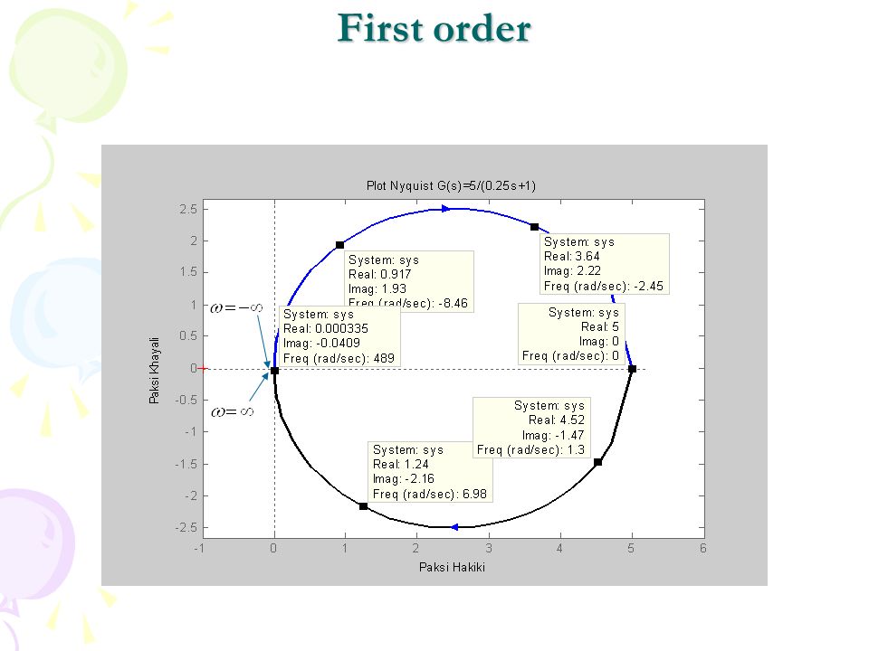
45. (i) At,,, and (ii) At, dan. i.e.or (iii) No crossing in the real axis as, (iv) No crossing in the imaginary axis as, is a circle. First order

46. Example: Nyquist plot of Frequency response and At and At, and,. >> nyquist([5],[.25 1]) First order

50. Second Order

51. Frequency response Rearrange

52. Magnitude Phase angle and (i) at, (ii) At, and. (iii) No crossing on the real axis. (iv) Crossing of the imaginary axis when,. and Second Order

53. Example: Frequency response Magnitude Phase angle Second Order

54. (i) At, (ii) At, and (iii) Real axis crossing at,, and rad.s -1 or Magnitude (iv) Imaginary crossing at =0.6 rad.s -1, Magnitude »dr1=[2 1]; » dr2=[1 1 1]; » dr=conv(dr1,dr2); » nr=1; » nyquist(nr,dr) Second Order,

56. Nyquist Path For Nyquist path  jj r s-plane Contour of which will give the closed loop poles for till by replacing to become jj  F(j  )-plane

57. However Hence on F(j  )-plane, we represent GH(j  )-plane to plot jj  -1+j0. Nyquist Path GH(j  )-plane

58. Nyquist Stability Criterion The criteria states that the number of closed poles of a system is equal to the number of open-loop, G(s)H(s), zeros plus the number of encirclements in the clockwise direction by the Nyquist plot of the open-loop, G(s)H(s). Or, it can be represented in mathematic form as where Z = Number of zeros on the right-half plane of j  -axis, where. N = Number of clockwise encirclement of P = Number of open-loop poles on the right-half plane of j  -axis.

59. Consider, applying the Nyquist stability criteria Z=N+P=1+0=1 Hence the system has 1 closed-loop pole on the right of the imaginary axis Example

60. s^2 + 10 s + 24 --------------- s^2 - 8 s + 15 Example The first thing we need to do is find the number of positive real poles in our open-loop transfer function, P: >>roots([1 -8 15]) ans = 5 3 The second thing we need to do is find the number of positive real zeros in our open-loop transfer function, Z: >>roots([1 10 24]) ans = -6.0000 -4.0000 Z=N+P N=Z-P=0-2=-2 The poles of the open-loop transfer function are both positive. Therefore, we need two anti- clockwise (N = -2) encirclements of the Nyquist diagram in order to have a stable closed- loop system (Z = P + N). If the number of encirclements is less than two or the encirclements are not anti-clockwise, our system will be unstable. Let's look at our Nyquist diagram for a gain of 1: nyquist([ 1 10 24], [ 1 -8 15])

61. Example

62. Stability analysis  There is no encirclement of the -1+j0 point. This implies that the system is stable if there are no poles of G(s)H(s) in the right-half s plane; otherwise, the system is unstable.  There are one or more counterclockwise encirclements of the -1+j0 point. In this case the system is stable if the number of counterclockwise encirclements is the same as the number of poles of G(s)H(s) in the right-half s plane; otherwise, the system is unstable.  There are one or more clockwise encirclements of the -1+j0 point. In this case the system is unstable. Nyquist Stability Criterion

63. Is the reciprocal of the magnitude at the frequency at which the phase angle is -180 0. Phase crossover frequency, Frequency where the phase angle of is –180 o Gain crossover frequency, Frequency where the magnitude of Gain margin, Gain margin in Nyquist Plot GH(j  )-plane jj  -1+j0 1/GM Gain margin,

64. Phase margin in Nyquist Plot jj  -1+j0 GH(j  )-plane Unit circle will give phase angle ofhence the phase margin Phase margin,

65. Negative gain and phase margins in Nyquist Plot -1+j0  jj GH(j  )-plane As, the gain margin As, the phase margin

66. For Example:, shows the Nyquist plot and its respective gain and phase margin + - Open loop transfer function Frequency response Example

67. Magnitude Phase angle (i) At, and (ii) At, and Example

68. Real crossing, when. (iii) then Imaginary crossing, when (iv) then » nr=40; » dr1=[ 1 3]; » dr2=[1 4 7]; » dr=conv(dr1,dr2); » nyquist(nr,dr) Example

69. Example

70. Example At  =2.54

71. Positive gain and Phase margins in Bode plot LM (dB)  (rad.s-1) 0 GM  0 o PM -180 o GM – gain margin PM – phase margin - Gain crossover frequency - Phase crossover frequency

72. Negative gain and Phase margins in Bode plot LM (dB) GM  (rad.s-1 ) PM 0  -180 o 0 o Note that, negative gain or phase margin means that the system is not stable

73. Example: If and K=96 determine gain and phase crossover frequencies. Consequently what is the system gain and phase margin. + - Example

74. Frequency response and Example

75. kutub orijin kutub hakiki (rad.s -1 )0.1240 (dB/dekad) -20 (dB/dekad) 0-20 (dB/dekad) 00-20 Total slope dB/decade -20-40-60 Table of LM slope for the 3 poles Example

76. kutub hakiki  (rad.s -1 ) 0.10.2420400 kecerunan (darjah/dekad) 0-45 00 kecerunan (darjah/dekad) 00-45 0 jumlah kecerunan (darjah/dekad) 0-45-90-450 Table for phase angle slope from the two poles, notes that the pole at origin does not contribute to the slope as the angle is constant -90 o Example

77. (rad.s -1 )0.12404001000 Total slope (dB/dec) -20-40-60 LM (dB)22-4-56-116-140 To obtain the LM vs freq. plot, we determine the LM value at the corner frequency, this can be obtained by simple trignometry (dB/dekad) Using the trignometry’s formula, Example

78. As for the LM slope, we apply a trignometry’s formula to obtain the phase angle slope at the low and high frequency for each corner frequency as in table below  (rad.s -1 ) 0.10.24204001000 Total slope (deg/dec) 0-45-90-4500 (deg) -90 -149-212-271 (deg/decade) Example

79. Example

80. >> bode([96],[1 42 80 0]) Example

81. >>[GM,PM,Wg,Wp] = margin(sys) Example

82. >> num=[96];den=[1 42 80 0]; >> sys=tf(num,den); >> [GM,PM,Wg,Wp] = margin(sys) Gm = 35.0000 Pm = 60.5601 Wg = 8.9443 Wp = 1.0599 >> Gm_dB = 20*log10(Gm) Gm_dB = 30.8814 Example