Download presentation
Presentation is loading. Please wait.

1
سیستمهای کنترل خطی پاییز 1389 بسم ا... الرحمن الرحيم دکتر حسين بلندي - دکتر سید مجید اسما عیل زاده

2
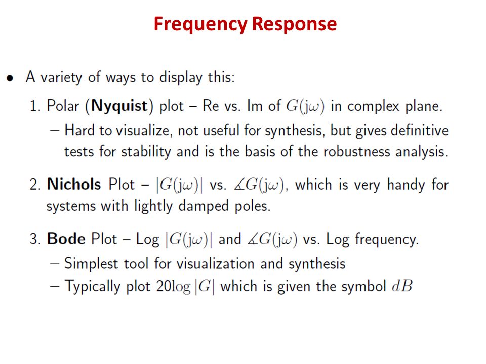
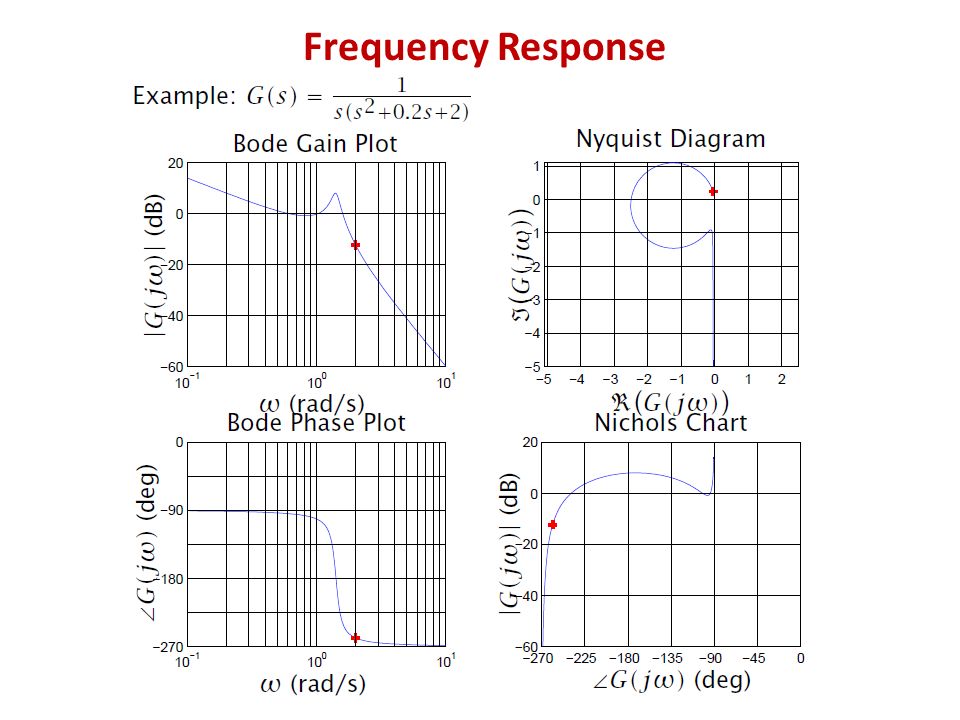
Frequency Response

6
Bode Form: Plot the asymptotic approximations for each term separately, for both magnitude and angle. Then add them together to get the system asymptotic approximation. Sketch in the Bode plot curve. )2)(5( )10(10 )( sss s s G )2/1)(5/1( )10/1( )2)(5( )10( )( jjj j jjj j j G method to plot the magnitude response of the Bode diagram
2)(5( )10(10 )( sss s s G )2/1)(5/1( )10/1( )2)(5( )10( )( jjj j jjj j j G method to plot the magnitude response of the Bode diagram.")
7
)2/1)(5/1( )10/1( jjj j
2/1)(5/1( )10/1( jjj j ")
8
method to plot the magnitude response of the Bode diagram

11
Bode Form: The damping ratio for the second-order term is = 0.1 and the natural frequency is 10 rad./s. 1002 1 5 )( 2 sss sG 2 2 10/ /2.01 1 1/1 5 1002 1 5 )( j j jj j jG method to plot the magnitude response of the Bode diagram
( 2 sss sG / / / )( j j jj j jG method to plot the magnitude response of the Bode diagram.")
12
2 2 10/ /2.01 1 1/1 5 1002 1 5 )( j j jj j jG
( j j jj j jG")
13
0dB, 0 o 100 10 10.10.1 20dB, 45 o -20dB, -45 o -40dB, -90 o 40dB, 90 o -80dB,-180 o -60dB.-135 o -100dB,-225 o -120dB,-270 o - 60dB/dec - 20dB/dec There is a resonant peak M r at: 1.25dB - 20dB/dec method to plot the magnitude response of the Bode diagram

14
Given: First: Always, always, always get the poles and zeros in a form such that the constants are associated with the jw terms. In the above example we do this by factoring out the 10 in the numerator and the 500 in the denominator. Second: When you have neither poles nor zeros at 0, start the Bode at 20log 10 K = 20log 10 100 = 40 dB in this case. wlg method to plot the magnitude response of the Bode diagram

15
1 1 1 (rad/sec) dB Mag Bode Plot Magnitude for 100(1 + jw/10)/(1 + jw/1)(1 + jw/500) 1 1 1 (rad/sec) dB Mag 0 20 40 -20 -60 60 -60 0.1 1 10 100 1000 10000
 dB Mag Bode Plot Magnitude for 100(1 + jw/10)/(1 + jw/1)(1 + jw/500) (rad/sec) dB Mag")
16
1 1 1 (rad/sec) 0 20 40 60 -20 -40 -60 1 10 100 10000.1 (rad/sec) dB Mag 0 20 40 60 -20 -40 -60 1 10 100 10000.1 Bode Plots Example : -20db/dec -40 db/dec The completed plot is shown below.
 (rad/sec) dB Mag Bode Plots Example : -20db/dec -40 db/dec The completed plot is shown below.")
17
1 1 1 (rad/sec) dB Mag Bode Plots Example: Given: 1 0.1 10 100 40 20 0 60 -20. 20 log80 = 38 dB -60 dB/dec -40 dB/dec

18
1 1 1 (rad/sec) dB Mag 0 20 40 60 -20 -40 -60 1 10 100 10000.1 Bode Plots -40 dB/dec + 20 dB/dec Given: Example: 2
 dB Mag Bode Plots -40 dB/dec + 20 dB/dec Given: Example: 2")
19
1 1 1 (rad/sec) dB Mag 0 20 40 60 -20 -40 -60 1 10 100 10000.1 Bode Plots -40 dB/dec + 40 dB/dec Given: Example
 dB Mag Bode Plots -40 dB/dec + 40 dB/dec Given: Example")
23
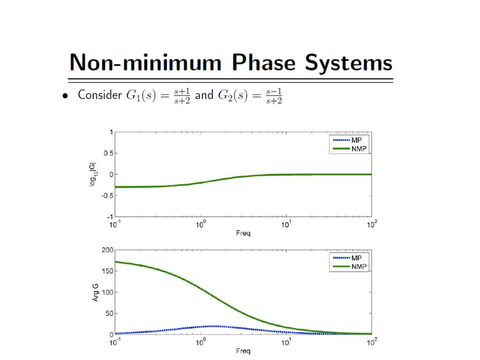
Determine the transfer function in terms of the Bode diagram The minimum phase system(or transfer function) We have: The magnitude responses are the same. But the net phase shifts are different when ω vary from zero to infinite. It can be illustrated as following: Sketch the polar plot: Compare following transfer functions:

24
Determine the transfer function in terms of the Bode diagram Compare following transfer functions: Only for the minimum phase systems we can affirmatively determine the relevant transfer function from the magnitude response of the Bode diagram.

25
2 20 200 0dB, 0 o 100 10 10.10.1 - 40dB/dec - 20dB/dec Determine the transfer function from the magnitude response of the Bode diagram Example : suppose the system is minimum phase

26
0dB, 0 o 100 10 1 0.10.1 - 180 o - 90 o - 20dB/dec Example All satisfy the magnitude response But Determine the transfer function from the magnitude response of the Bode diagram

27
Transfer Function Identification Frequency response characteristics can be be obtained experimentally by applying sinusoidal inputs of various frequencies, and measuring the gain and phase relationships between input and output. By fitting asymptotic approximations to the frequency response characteristics obtain from experimental measurements, an approximate transfer function model of the system can be obtained.

28
Transfer Function Identification: Transfer Function Identification: Major Steps 1. Determine the initial slope order of poles at the origin. 2. Determine the final slope difference in order between the denominator and numerator (n m). 3. Determine the initial and final angle confirm the results from above or detect the presence of a non-minimum phase system (delays or zeroes in the RHS). 4. Determine the low frequency gain (Bode gain).
. 3. Determine the initial and final angle confirm the results from above or detect the presence of a non-minimum phase system (delays or zeroes in the RHS). 4. Determine the low frequency gain (Bode gain)..")
29
5. Detect the number and approximate location of corner frequencies and fit asymptotes. – examine expected -3dB points. – try to separate second-order terms and use the standard responses to estimate damping. 6. Sketch the phase plot for the identified transfer function as a check of accuracy. Transfer Function Identification: Transfer Function Identification: Major Steps

30
7. Use the phase plot to check for non-minimum phase terms and to calculate the time delay value if one is present. 8. Calculate the frequency response for the identified model and check against the experimental data (MatLab or a few points by hand calculation). 9. Iterate and refine the pole/zero locations and damping of second-order terms. Transfer Function Identification: Transfer Function Identification: Major Steps
. 9. Iterate and refine the pole/zero locations and damping of second-order terms. Transfer Function Identification: Transfer Function Identification: Major Steps.")
31
)2)(5( )10(10 )( sss s sG Example Example I:
2)(5( )10(10 )( sss s sG Example Example I:")
32
Initial slope = 20dB/dec. a 1/ j term. Final slope = 40dB/dec. ( n-m ) = 2. Initial angle = 90 and the final angle is 180 which checks with the gain curve. Low frequency gain is found to be | K B / | dB = 35dB, where = 0.1 K B = 5.62. Through asymptotic fitting there are two poles found at c = 4 and 25, and one zero at c = 70.
 = 2. Initial angle = 90 and the final angle is 180 which checks with the gain curve. Low frequency gain is found to be | K B / | dB = 35dB, where = 0.1 K B = Through asymptotic fitting there are two poles found at c = 4 and 25, and one zero at c = 70..")
33
+45 /dec.

34
The estimated transfer function in Bode form is The final form is )25)(4( )70(8 )( sss s sG )25/1)(4/1( )70/1(62.5 )( jjj j jG
25)(4( )70(8 )( sss s sG )25/1)(4/1( )70/1(62.5 )( jjj j jG ")
35
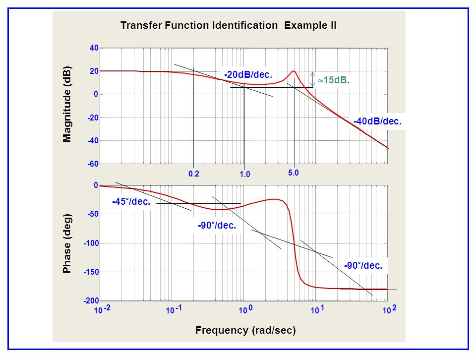
Example Example II:

36
Initial slope = 0dB/dec. no pole at the origin. Final slope = 40dB/dec. (n-m) = 2. Initial angle = 0 and the final angle is 180 which checks with the gain curve. Low frequency gain is found to be |K B | dB = 20dB K B = 10. Through asymptotic fitting a simple pole is found at c = 0.2, a simple zero at c = 1.0 and a complex pole at n = 5.0.
 = 2. Initial angle = 0 and the final angle is 180 which checks with the gain curve. Low frequency gain is found to be |K B | dB = 20dB K B = 10. Through asymptotic fitting a simple pole is found at c = 0.2, a simple zero at c = 1.0 and a complex pole at n =")
38
The peak at n = 5.0 is 15dB which corresponds to a damping ratio of 0.1. The estimated transfer function in Bode form is The final form is )25)(2.0( )1(50 )( 2 sss s sG )25/5/2.01)(2.0/1( )1/1(10 )( 2 jj j jG
25)(2.0( )1(50 )( 2 sss s sG )25/5/2.01)(2.0/1( )1/1(10 )( 2 jj j jG .")
39
Bode Plots Design Problem: Design a G(s) that has the following Bode plot. dB mag rad/sec 0 20 40 0.11101001000 30900 30 dB +40 dB/dec - 40dB/dec ?? Example

40
Bode Plots Procedure: The two break frequencies need to be found. Recall: #dec = log 10 [w 2 /w 1 ] Then we have: ( #dec )( 40dB/dec) = 30 dB log 10 [30/w 1 ] = 0.75 w 1 = 5.33 rad/sec Also: log 10 [w 2 /900] (-40dB/dec) = - 30dB This gives w 2 = 5060 rad/sec
( 40dB/dec) = 30 dB log 10 [30/w 1 ] = 0.75 w 1 = 5.33 rad/sec Also: log 10 [w 2 /900] (-40dB/dec) = - 30dB This gives w 2 = 5060 rad/sec.")
41
Bode Plots Procedure: Clearing: Use Matlab and conv: N = conv(N1,N2) N1 = [1 10.6 28.1] N2 = [1 10120 2.56e+7] 1 1.86e+3 2.58e+7 2.73e+8 7.222e+8 s 4 s 3 s 2 s 1 s 0
![Bode Plots Procedure: Clearing: Use Matlab and conv: N = conv(N1,N2) N1 = [ ] N2 = [ e+7] e e e e+8 s 4 s 3 s 2 s 1 s 0](http://images.slideplayer.com/23/6854371/slides/slide_41.jpg "Bode Plots Procedure: Clearing: Use Matlab and conv: N = conv(N1,N2) N1 = [ ] N2 = [ e+7] e e e e+8 s 4 s 3 s 2 s 1 s 0")
42
Bode Plots Procedure: The final G(s) is given by; Testing: We now want to test the filter. We will check it at = 5.3 rad/sec And = 164. At = 5.3 the filter has a gain of 6 dB or about 2. At = 164 the filter has a gain of 30 dB or about 31.6. We will check this out using MATLAB and particularly, Simulink.

43
Matlab (Simulink) Model:
 Model:")
44
Filter Output at = 5.3 rad/sec Produced from Matlab Simulink

45
Filter Output at = 70 rad/sec Produced from Matlab Simulink vvv

46
Consider the definitions of the gain and phase margins in relation to the Bode plot of GH ( j ). Gain Margin: the additional gain required to make | GH ( j ) | = 1 when / GH ( j ) = 180 . On the Bode plot this is the distance, in dB, from the magnitude curve up to 0 dB when the angle curve crosses 180 . Phase Margin: the additional phase lag required to make / GH ( j ) = 180 when | GH ( j ) | = 1. On the Bode plot this is the distance in degrees from the phase curve to 180 when the gain curve crosses 0 dB.
 | = 1 when / GH ( j ) = 180 . On the Bode plot this is the distance, in dB, from the magnitude curve up to 0 dB when the angle curve crosses 180 . Phase Margin: the additional phase lag required to make / GH ( j ) = 180 when | GH ( j ) | = 1. On the Bode plot this is the distance in degrees from the phase curve to 180 when the gain curve crosses 0 dB..")
47
)25)(4( )70(8 )( sss s sG
25)(4( )70(8 )( sss s sG")
52
2

Similar presentations


 Hany Ferdinando Dept. of Electrical Engineering Petra Christian University.>")


