Download presentation
Presentation is loading. Please wait.

1
Objective Digital Analog Forecasting “Is The Future In The Past?”

2
We’re Going Back ….. Back to the Future

3
Pattern Recognition Important to recognize the shape and influence of patterns and teleconnection indices. Teleconnections: AO, NAO, NAM, PNA, AAO, EA, WP, EP, NP, EAWR, SCA, POL, PT, SZ, ASU, PDO, El Nino/La Nina MEI, SOI, Nino1, Nino2, Nino3, Nino4, Nino3.4 Complex interactions in the mid and high latitudes makes forecasting most teleconnection indices difficult beyond a week or two.

4
55-yr Monthly Temporal Correlation of AO and 1000-500 mb Thickness

5
55-yr Monthly Temporal Correlation of AO and Precipitation

6
55-yr Monthly Temporal Correlation of AO and 500 mb Zonal Wind

7
55-yr Monthly Temporal Correlation of NAO and Surface Temperature

8
55-yr Monthly Temporal Correlation of PNA and 1000-500 mb Thickness

10
55-yr Monthly Temporal Correlation of MEI and 1000-500 mb Thickness

11
55-yr Monthly Temporal Correlation of MEI and Precipitation

12
Analog Motivation Monthly/seasonal pattern evolution affected by? Sea surface temperature anomalies ENSO Snow Cover / Icepack Solar cycle Phytoplankton Vegetation Atmospheric Chemistry Stratospheric Phenomena

13
Analog forecasting The oldest forecasting method? Compare historical cases to existing conditions Previous analog forecasting research yielded limited success New digital age of analog forecasting 1. Dataset availability 55 Year NCEP Reanalysis 40 Year ECMWF Reanalysis 109 Year Climate Division Data Etc 2. Computational resources – statistical forecasting - ensembling

14
A sobering perspective… “…it would take order 10 30 years to find analogues that match over the entire Northern Hemisphere 500mb height field to within current observational error.” From: Searching for analogues, how long must we wait? Van Den Dool, 1994, Tellus.

15
Goals Not seeking exact replication of patterns Instead, determine sign of the climatological departure using an analog ensemble (on a weekly to monthly time scale) Analogs require keys keys to matching keys to extracting Statistically extracting information relevant to current patterns and removing noise.
 Analogs require keys keys to matching keys to extracting Statistically extracting information relevant to current patterns and removing noise.")
16
Analog Components 1. Data Dataset length, frequency, area, variables, filtering 2. Matching Method Parameters, region, search window, threshold method (MAE, anomaly correlation, RMSE, etc), statically or dynamically 3. Ensemble Configuration Match/date selection, top (1,10,100,1000 matches), ensemble of single match analysis / ensemble of match analyses / both 4. Forecast Forecasts made from dates acquired from matching Integrate historical dates forward in time to generate ensemble forecast – mean, probabilistic distributions
, statically or dynamically 3. Ensemble Configuration Match/date selection, top (1,10,100,1000 matches), ensemble of single match analysis / ensemble of match analyses / both 4. Forecast Forecasts made from dates acquired from matching Integrate historical dates forward in time to generate ensemble forecast – mean, probabilistic distributions.")
17
Example Analog Forecasts 1. Seasonal tropical thickness forecasts 2. Seasonal San Diego precipitation forecasts 3. 2-4 week mid-latitude forecasts

18
Seasonal Tropical (20N-20S) Analog Thickness Forecasts
 Analog Thickness Forecasts")
19
1000-500hPa Thickness as Pattern Descriptor Fewer degrees of freedom (Radinovic 1975) Great integrator of: Long wave pattern Global temperature pattern Global lower tropospheric moisture pattern Large inertia: Not greatly influenced by transient fluctuations (e.g. short-lived convection)
.")
20
Matching Method? Instantaneous (unfiltered) thickness analyses? Filtered thickness analyses? Choice likely depends on desired forecast length Short term forecast: compare instantaneous analyses Long term forecast:compare filtered analyses Optimal Filtering F = f( t,L) t = forecast length (lead time) L = verification increment (hour, month, season)
 t = forecast length (lead time) L = verification increment (hour, month, season).")
21
Filtering Seasonal forecasting 30-day lagged mean smoothed thickness

22
Matching Window for July 1 JD 2003 JD 2002 JD 2001 JD 1948 JD 1949 JD JD JD JD JD Match exact time/date # = 55 Match within 2 wk window # 3000 JD JD JD JD JD Match allowed over entire year # 80000 2003 2002 2001 1948 1949

23
Analog selection for 00 UTC 12 January 2001. Choose the top 200 (out of 3000 possible or 6%) matches from a 2-week window around the initialization date. Exclude matching between the year before and after the initialization Consensus forecast made for each 6-hour initialization time in 1948-1998, approx 80,000 forecasts.
 matches from a 2-week window around the initialization date. Exclude matching between the year before and after the initialization Consensus forecast made for each 6-hour initialization time in , approx 80,000 forecasts..")
24
51 years of Analog Selection: The DNA of atmospheric recurrence? PercentPercent

25
Skill? Persistence, anomaly persistence? Convention for seasonal forecasting: Climatology. 54-year mean?10-year mean? 30-year mean?Previous year? Tropical (20°S-20°N) monthly mean thickness forecast is evaluated Skill = MAE CLIMO - MAE ANALOG
 monthly mean thickness forecast is evaluated Skill = MAE CLIMO - MAE ANALOG.")
26
Analog Forecast Skill: 51 year mean Skill to 8.5 months Skill to 25 months Skill to 12 months

27
Winter/spring 1997 Forecast of 1998 El Nino Pinatubo hinders analog matching Spring 1982 prediction of 1983 El Nino 2 Skill (shaded) = MAE CLIMO – MAE ANALOG : [Red: Skill > 2m ]
![Winter/spring 1997 Forecast of 1998 El Nino Pinatubo hinders analog matching Spring 1982 prediction of 1983 El Nino 2 Skill (shaded) = MAE CLIMO – MAE ANALOG : [Red: Skill > 2m ]](http://images.slideplayer.com/26/8533430/slides/slide_27.jpg "Winter/spring 1997 Forecast of 1998 El Nino Pinatubo hinders analog matching Spring 1982 prediction of 1983 El Nino 2 Skill (shaded) = MAE CLIMO – MAE ANALOG : [Red: Skill > 2m ]")
29
Seasonal Precipitation Forecasts

30
“Dependent” Analog Forecasts Analogs allow for forecasts of any dependent variable which has a historical record, regardless of what is matched. Forecasts of dependent variables requires some relationship to the matching parameter For example – electrical usage – long term record of electrical usage could be determined from dates provided by thickness matching, thanks to the dependence of electricity on temperature, and temperature on thickness.

31
Precipitation Forecasts Need an analog ensemble of matching dates Acquired from global thickness matching Daily historical records of surface parameters with a period as long as that from which the analogs matches were extracted 51 years (1948-1998)
")
32
MEI and Precipitation Correlation With Available GSN Data

33
Method San Diego precipitation forecasts Global thickness matching dates Surface precipitation observations Forecast length (1- 365) days Forecasts averaged over the length of period which is to be forecast e.g., a seasonal (3 month) forecast is composed of an average of 3 months of 6 hourly forecast initializations (~360 forecasts)
 days Forecasts averaged over the length of period which is to be forecast e.g., a seasonal (3 month) forecast is composed of an average of 3 months of 6 hourly forecast initializations (~360 forecasts)")
34
1983 El Nino1998 El Nino

35
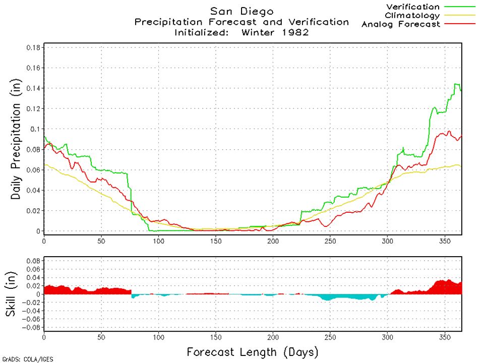
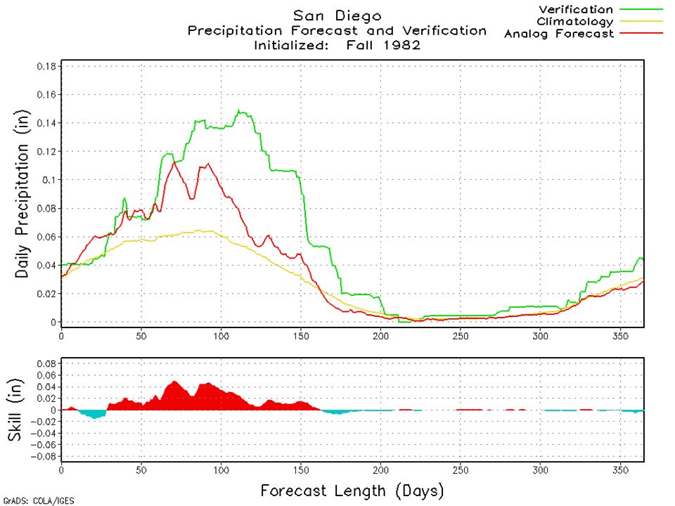
Seasonal Precipitation Forecast For San Diego Initialized 1982

40
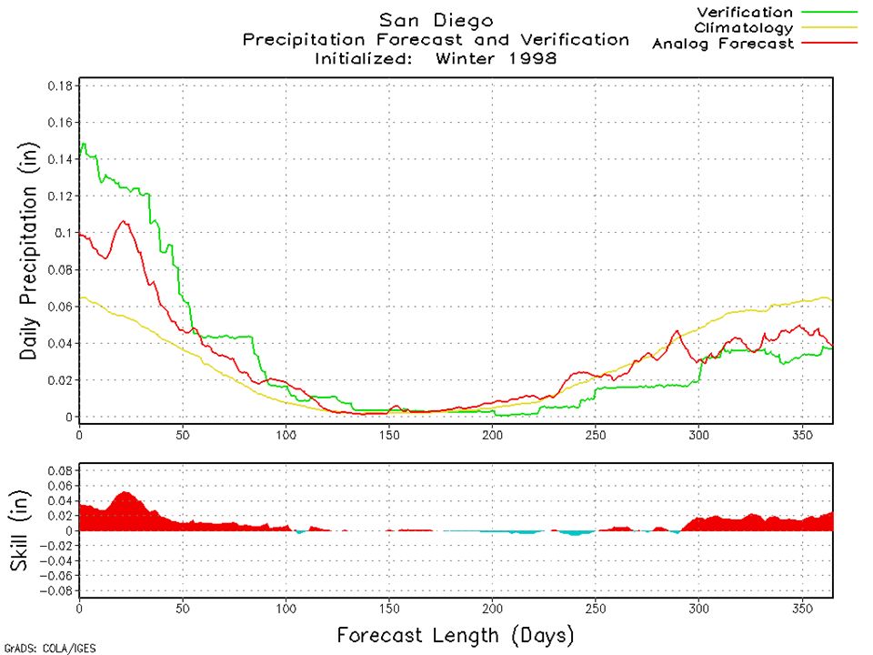
Seasonal Precipitation Forecast For San Diego Initialized 1997

45
Mid-Latitude 2-4 Week Thickness Forecasts

46
Method Technique similar to seasonal tropical forecasts with the following exceptions: 1-day filtered thickness analyses NH matching Matching window - 4 weeks Forecast length 1-30 days

47
Observed Analyses 00Z14MAR1993 Analog Ensemble Size Analog Ensemble Consensus Top (1,10,100,500 analogs) 00Z14MAR1993
 00Z14MAR1993")
48
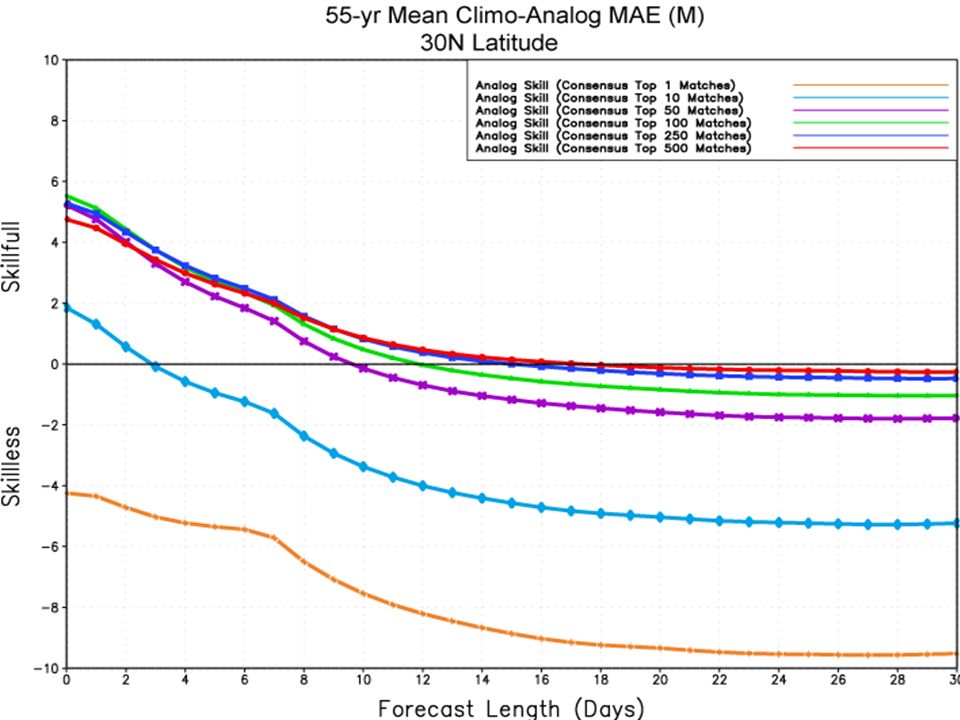
Optimal Analog Ensemble Size at Analysis

51
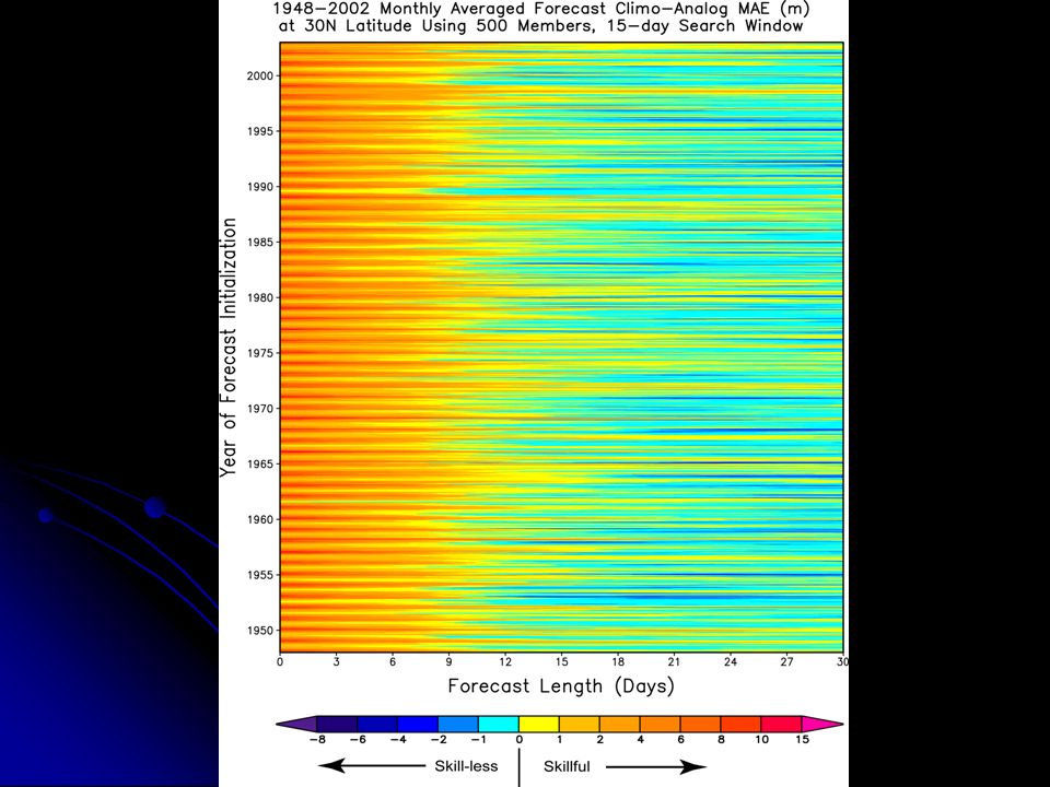
Analog Skill Length as a Function of Year and Season

52
Forecast Skill Variability Distinct periods where analog forecast skill extends to 30 days or beyond ENSO Blocking Well represented patterns - good analogs Forecast confidence?

53
Example Forecast 00Z15JAN1995 Analysis Week 1 Week 2 Week 3

54
A flood of unanswered questions… How does analog forecast skill vary with filtering of thickness in time and space What is the impact of using another reanalysis dataset (ECMWF, JMS)? How will mutli-parameter analogs impact skill? Will temporal sequence matching vs static matching improve analog selection? Can we blend dynamical prediction systems with analogs to further improve the skill of both?

Similar presentations


 is responsible for forecasts several times.>")
