1. Discrete-time controllers structures and tuning Š. Kozák 2000, Department of Automatic Control Systems For Vienna University

2. PID regulátory – spätnoväzbové štruktúry Riadenie (CO) u(t) : Proportional gain Integral gain Derivative gain

3. Proportional feedback gain K P Proportional control : Feedback control c(t) is linearly proportional to the error : Steady state error will decrease Faster response Too much gain will make the system unstable

4. Integral feedback gain K I Integral control: Penalty on the past error Zero steady state error Destabilizing influence –It gets oscillatory as K I increases

5. Derivative feedback gain K D Derivative control: Stabilize the system: –reduce oscillatory behavior Create a damping effect in the system dynamics It makes system slow down

6. Continuous regulator: principle of PID set-point plant command variable KiKi KpKp KdKd dd d dt PID The proportional factor K p generates an output proportional to the error, it requires a non- zero error to produce the command variable. Increasing the amplification Kp decreases the error, but may lead to instability The integral factor K i produces a non-zero control variable even when the error is zero, but makes response slower. The derivative factor K d speeds up response by reacting to an error step with a control variable change proportional to the step. error process value integral factor derivative factor proportional factor measurement

7. PID response asymptotic error: proportional only too much proportional factor: unstable no remaining error, but sluggish response: integral only differential factor increases responsiveness

8. Performance specifications of the closed loop system (step response ) Steady state error: Maximum overshoot: Delay time: Rise time: Settling time:

9. Digital control systems Digital realisation of an “analogue type” controller ADC- Digital controller - DAC should behave the same as an analogue controller (e.g. PID type), which implies the use of a high sampling frequency (the algorithm implemented is very simple) Bad use of the potentialities of the digital controller System Digital Controller y(t) Perturbations e  t) y ref (t) + - DACADC e  k) u(k) u(t) TsTs “Il ne suffit pas de mettre un TIGRE (microprocesseur ou DSP) dans son régulateur, il faut rajouter de l’intelligence”

10. System Digital Controller y(t) Perturbations Yref(k) + - DAC e(k) u(k) u(t) Ts The sampling frequency is chosen in accordance with the bandwidth desired for the closed-loop system Intelligent use of the “computer” : high sampling period and then implementation of complex algorithms requiring greater computation time. Not only a copy of analogue control : BRAINWARE The sampling frequency is chosen in accordance with the bandwidth desired for the closed-loop system Intelligent use of the “computer” : high sampling period and then implementation of complex algorithms requiring greater computation time. Not only a copy of analogue control : BRAINWARE ADC y(k) Discretized System Digital control systems Discrete-time system models and digital control algorithms y(k) = f[y(k-i), u(k-j)] or G(z -1 ) = z -d B(z -1 )/A(z -1 )

11. Choice of sampling frequency fs = 1/Ts = (6 to 25) * f CL B fs : sampling period f CL B : bandwidth of the closed-loop system fs = 1/Ts = (6 to 25) * f CL B fs : sampling period f CL B : bandwidth of the closed-loop system If fs is fixed => limit for f CL B (  fs /15 ) No more

12. Úvod do prepočtov spojitých regulátorov na diskrétne formy Ideálne „textbook“ PID regulátory Neideálne formy a opisy PID regulátorov Podmienky ekvivalentnosti spojitých a diskrétnych PID regulátorov vzhľadom na periódu vzorkovania Rekurentné formy – diferenčné rovnice diskrétnych PID regulátorov PID regulátory s ohraničením riadiaceho zásahu

13. Neidealizovaný (reálny) PID regulátor obsahuje v derivačnej zložke oneskorovací člen (zabezpečujúci realizovateľnosť derivačnej zložky). Základné spojité formy PID regulátorov Neideálna forma opisu PID (realizovateľná) ff =T d *(1/T f *Dirac(t)-1/T f 2 *exp(-t/T f ))

14. Základné diskrétne formy opisu PID regulátora Prenosová funkcia diskrétneho regulátora v s a z-oblasti : 2. 1.

15. ff =T d *(1/T f *Dirac(t)-1/T f 2 *exp(-t/T f )) Doplnok : Ako určiť originál k derivačnej zložke

16. 1. Ak nahradíme integrál v spojitej verzii sumou (obdlžníková náhrada) deriváciu diferenciou prvého rádu, potom v k-tom diskrétnom kroku riadiaci zásah je vyjadrený kde P - je koeficient zosilnenia odpovedajúci proporcionálnemu zosilneniu spojitého PID regulátora, T i – resp. T d sú koeficienty odpovedajúce integračnej resp. derivačnej časovej konštante spojitého regulátora Rekurentný vzťah pre riadiaci zásah sa určí rozdielom u(k)-u(k-1) k k-1 - odčítaním Základné diskrétne formy PID regulátorov (DPID)

17. q0q0 q1q1 q2q2 q 0 > 0 q 1 >- q 0 -(q 0 +q 1 ) < q 2 < q 0 Podmienky ekvivalentnosti :

18. q0q0 u(k) q 0 -q 2 2q 0 +q 1 t=kT q 0 +q 1 + q 2 PCH - PID REGULÁTORA-PODM.EKVIVALENTNOSTI q 0 > 0 q 1 >-q 0 -(q 0 +q 1 ) < q 2 < q 0

19. K(1+c d ) u(k) K K(1+c i ) t=kT Kc i PCH - PID REGULÁTORA-PODM.EKVIVALENTNOSTI c d > 0 c i > 0 c i < c d

20. u(k) q0q0 t=kT PCH - PI REGULÁTORA-PODM.EKVIVALENTNOSTI q 0 +q 1

21. w(k)=w(k-1)=w(k-2) Iné formy a vyjadrenia diskrétneho PID regulátora Takahashiho vzťah (feedforward forma diskrétneho PID-u):

22. q0q0 q1q1 q2q2 - 2. Ak nahradíme integrál v spojitej verzii sumou (lichobežníková náhrada) deriváciu diferenciou prvého rádu, potom v k-tom a k-1 diskrétnom kroku riadiaci zásah je vyjadrený

23. Prenosová funkcia diskrétneho PID regulátora

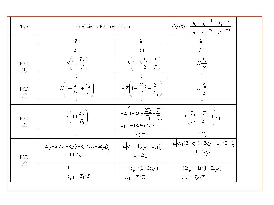
24. Podmienky ekvivalentnosti PID a PSD regulátora Podmienky „ekvivalentnosti“:

25. q0q0 u(k) q 0 -q 2 2q 0 +q 1 t=kT q 0 +q 1 + q 2 q 0 > 0 q 1 >-q 0 -(q 0 +q 1 ) < q 2 < q 0

26. Podmienky ekvivalentnosti PSD regulátora s PID regulátorom Iná ekvivalentná forma vyjadrenia diskrétneho PID regulátora (rkoz0)

27. Veľmi často sa odchýlka nahrádza e(k) e(k-1), čím sa dosahuje okamžité pôsobenie riadiaceho zásahu na proces. Táto zmena sa prejaví aj v prenosovej funkcii regulátora na integračnej zložke, ktorá neobsahuje v čitateli člen z -1. Integračná zložka: Riadiaci zásah podľa (rkoz0) je potom tvorený súčtom jednotlivých zložiek Derivačná zložka : Proporcionálna zložka : Paralelná forma diskrétneho PID regulátora: Upravený tvar DPID

28. Vynechávaním jednotlivých koeficientov q i, pre i=0,1,2 dostaneme rôzne štruktúry diskrétnych regulátorov. Ak vo vzťahu (rkoz0) položíme q2=0, dostaneme prenosovú funkciu diskrétneho regulátora v tvare: Diskrétny regulátor opísaný vzťahom (rkoz1) voláme diskrétny regulátor prvého rádu (PS-regulátor). Riadiaci zásah diskrétneho PI regulátora je vyjadrený diferenčnou rovnicou (rkoz1) Podmienky ekvivalentnosti sú odvodené podobne ako u PID regulátora

29. u(k) q0q0 t=kT PCH - PI REGULÁTORA-PODM.EKVIVALENTNOSTI q 0 +q 1

30. Iné vyjadrenie PS regulátora je možné pomocou koeficientov K, c i a c d. Pre q 2 =0 je zosilnenie K a koeficienty c d a c i vyjadrené Prenosová funkcia diskrétneho PI regulátora (DPI) použitím koeficientov K, c i : Riadiaci zásah

31. Diskrétny I regulátor získame ak položíme q 0 =0, q 2 =0. Prenosová funkcia diskrétneho I regulátora je v tvare: Riadiaci zásah určíme z prenosovej funkcie Ak položíme c i =0, dostaneme diskrétny PD regulátor s prenosovou funkciou: Prenosová funkcia diskrétneho P regulátora Riadiaci zásah P regulátora: u(k) = q 0 e(k) ?

32. Modifikácia PID regulátorov úpravou derivačného člena jednoduchá náhrada derivácie diferenciou prvého rádu vnáša nepresnosti do rekurzívnzych a nerekurzívnzych foriem PSD regulátorov a môže spôsobiť, že riadiaci zásah nadobúda veľké a prudké zmeny. Aby sa tomu predišlo, využíva sa náhrada derivácie priemernou hodnotou napr. zo štyroch hodnôt odchýlky: Ak použijeme nerekurzívnu formu PID regulátora, potom deriváciu nahradíme vzťahom : pre rekurentnú formu:

33. PID formy „neidealizovaného“ diskrétneho regulátora Ak spojitý PID regulátor obsahuje v derivačnej zložke oneskorovací člen, môžeme jeho diskrétny opis určiť niekoľkými spôsobmi. Prakticky sa využívajú dva spôsoby prepočtu: Prvý spôsob prepočtu je realizovaný na základe určenia z-obrazu zo spojitého opisu, t.j.

34. Druhý spôsob výpočtu parametrov PID neideálneho diskrétneho PID regulátora môžeme určiť aproximatívnym spôsobom podľa Tustinového vzťahu. Dosadením za

35. Riadiaci zásah PID(NI) regulátora

37. Doplnok – kvalita regulácie frekvenčná oblasť

38. Closed Loop Open loop : system H(s) ; system with controller F(s).H(s) Closed loop : H CL (s) = F(s).H(s) / [ 1 + F(s). H(s) G(s) ] G(s) System Reg. Transducer F(s) H(s) Yref Y Disturbances Perturbations  + - Feed P Steady state error : F(s) must contains the internal model of the reference (the transfer function that generates Yref(t) from the Dirac impulse ; e.g. step = (1/s) * Dirac ; ramp = (1/s 2 ) * Dirac,...

39. Closed Loop : Perturbation rejection Perturbation-output sensitivity function : S yp (s) = Y(s) / P(s) = 1 / [1 + F(s).H(s).G(s)] Perturbation-output sensitivity function : S yp (s) = Y(s) / P(s) = 1 / [1 + F(s).H(s).G(s)] Perturbation rejection : S yp (0) = 0 to get a perfect rejection of the perturbation in steady state (controller must contain the classes of perturbation) and |S yp (  ) | < G ;   [ Example : |S yp (  ) | < 2 (6dB) ;   If the energy of the perturbation is concentrated in a given frequency band, the |S yp (  ) | should be limited in this band. Perturbation rejection : S yp (0) = 0 to get a perfect rejection of the perturbation in steady state (controller must contain the classes of perturbation) and |S yp (  ) | < G ;   [ Example : |S yp (  ) | < 2 (6dB) ;   If the energy of the perturbation is concentrated in a given frequency band, the |S yp (  ) | should be limited in this band.

40. Controller Design In order to design and tune a controller : 1) To specify the desired control loop performances Regulation and tracking : rise time and max overshoot or bandwidth and resonance 2) To choose a suitable controller design method 3) To know the dynamic model of the plant to be controlled => control model In order to design and tune a controller : 1) To specify the desired control loop performances Regulation and tracking : rise time and max overshoot or bandwidth and resonance 2) To choose a suitable controller design method 3) To know the dynamic model of the plant to be controlled => control model Control model : - Non parametric models : e.g. frequency response, step response,… - Parametric models : e.g. transfer function, differential eq., state eq. To get the model : - knowledge type model (based on the physic laws) ; used for plant simulation and design - identification models (from experimental data)

41. Continuous - time Models : Frequency Domain Linear system System u(t) = e j  t u(t) = e st y(t) = G(j  ). e j  t y(t) = G(s). e st  or f 20.log(|G|) Gain Phase  or f deg Bode Diagram x x xo Root locus : poles and zeroes Nyquist, Nichols,... Note: State Equation Differential Eq. Transfer function Observability, Controlablity

42. Continuous - time Models : Time responses Response of a dynamic system for a step input t Final Value (Steady state) Maximum overshoot (M) tRtR ts 0.9 FV t R : Rise Time ; define as the time needed to attain 90% of the final value ; or as the time needed for the output to pass from 10 to 90% of the final value t S : Settling Time ; define as the time needed for the output to reach and remain within a tolerance zone around the final value (±10%, ± 5%, ±1%,…) FV : Final Value ; a fixed output value obtained for t   M : Maximum Overshoot ; expressed as a percentage of the final value Example : 1 st Order H(s) = G/(1+sT) FV = G t R = 2.2 T t S = 2.2 T (for 10% FV) t S = 3 T ( for 5% FV) M = 0

43. Continuous - time Models : Frequency responses f B : Bandwidth ; the frequency from which the zero-frequency (steady state) gain G(0) is attenuated by more than 3 dB ; G(w B ) = G(0) - 3dB or G(w B ) = 0.707. G(0) f C : Cut-off frequency ; the frequency from which the attenuation is more than N dB ; G(w C ) = G(0) - NdB Q : Resonance factor ; the ratio between the gain corresponding to the maximum of the frequency response curve and the value G(0) f B : Bandwidth ; the frequency from which the zero-frequency (steady state) gain G(0) is attenuated by more than 3 dB ; G(w B ) = G(0) - 3dB or G(w B ) = 0.707. G(0) f C : Cut-off frequency ; the frequency from which the attenuation is more than N dB ; G(w C ) = G(0) - NdB Q : Resonance factor ; the ratio between the gain corresponding to the maximum of the frequency response curve and the value G(0) 20 log[ H(jw) ] w= 2 p f Resonance - 3 dB w B (f B ) w C (f C ) (p - m) x 20 dB/dec Nb of poles Nb of zeroes N dB

44. Reciprocity : Time / Frequency - 3 dB f B = 1/(2  T) f B  0.35 / t R 0.1 0.9 t R = 2.2 T time frequency

45. Closed Loop : Margins  Im H(j  )  Re H(j  ) 1/G Gain Margin : DG = 1 / |H(jw 180 )| for F(w 180 ) = -180  Typical : G  2 (6dB) [min: 1.6 (4dB)] Gain Margin : DG = 1 / |H(jw 180 )| for F(w 180 ) = -180  Typical : G  2 (6dB) [min: 1.6 (4dB)]  Phase Margin :  = 180  -  (  cr ) for |  (j  cr ) = 1  cr : crossing pulsation Typical : 30     60  Phase Margin :  = 180  -  (  cr ) for |  (j  cr ) = 1  cr : crossing pulsation Typical : 30     60   cr Delay Margin :  =  0.  cr additional delay that could be tolerate by the open loop system without instability for the closed loop system Delay Margin :  =  0.  cr additional delay that could be tolerate by the open loop system without instability for the closed loop system  Module Margin :  M = |1 + H(j  )| min = |S -1 yp (j  )| min Measure of perturbation rejection and robustness of non linearity and time variable parameters Typical :  M  0.5 (-6dB) [min: 0.4 (-8dB)] Module Margin :  M = |1 + H(j  )| min = |S -1 yp (j  )| min Measure of perturbation rejection and robustness of non linearity and time variable parameters Typical :  M  0.5 (-6dB) [min: 0.4 (-8dB)]