1. Discrete Controller Design
Chapter 9:
Discrete Controller Design
(PID Controller)

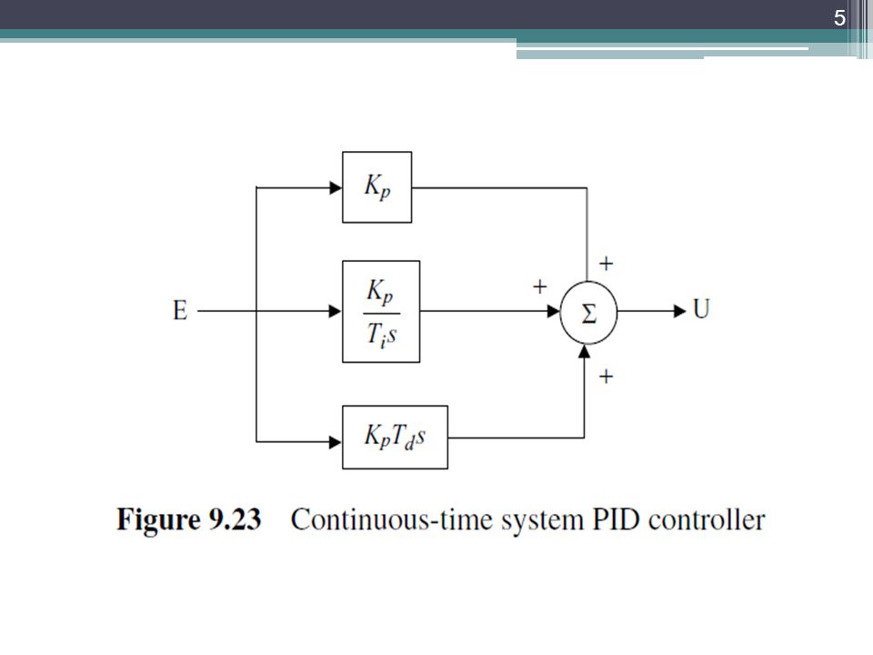
2. 9.2 PID CONTROLLER
The proportional–integral–derivative (PID) controller is often referred to as a ‘three-term’ controller.
It is one of the most frequently used controllers in the process industry.
In a PID controller the control variable is generated from the sum of a term proportional to the error, a term which is the integral of the error, and a term which is the derivative of the error.

3. 9.2 PID CONTROLLER
Proportional: the error is multiplied by a gain Kp. A very high gain may cause instability, and a very low gain may cause the system to be very sluggish (slow).
Integral: the integral of the error is found and multiplied by a gain. The gain can be adjusted to drive the error to zero in the required time.
Derivative: The derivative of the error is multiplied by a gain. The derivative control is used to improve the transient response by reducing overshoot.

4. The input–output relationship of a PID controller can be expressed as
where u(t) is the output from the controller and e(t) = r (t) − y(t), in which r (t) is the desired set-point (reference input) and y(t) is the plant output. Ti and Td are known as the integral and derivative action time, respectively.
By taking the Laplace transform of this equation, we can write the transfer function of a continuous-time PID as

6. Discrete PID Controller
To implement the PID controller using a digital computer we have to convert the equation:
from a continuous to a discrete representation.
There are several methods for doing this and the simplest is to use the trapezoidal approximation for the integral and the backward difference approximation for the derivative:
0 𝑡 𝑒 𝑡 𝑑𝑡 ≈ 𝑘=1 𝑛 𝑇𝑒 𝑘𝑇 , 𝑑𝑒(𝑡) 𝑑𝑡 ≈ 𝑒 𝑛𝑇 −𝑒(𝑛𝑇−𝑇) 𝑇

7. Using these approximations, we can write:
𝑢 𝑛𝑇 = 𝐾 𝑝 [𝑒 𝑛𝑇 + 1 𝑇 𝑖 𝑘=1 𝑛 𝑇𝑒 𝑘𝑇 + 𝑇 𝑑 𝑒 𝑛𝑇 −𝑒(𝑛𝑇−𝑇) 𝑇 ],
𝑢 𝑛𝑇−𝑇 = 𝐾 𝑝 [𝑒 𝑛𝑇−𝑇 + 1 𝑇 𝑖 𝑘=1 𝑛−1 𝑇𝑒 𝑘𝑇 + 𝑇 𝑑 𝑒 𝑛𝑇−𝑇 −𝑒(𝑛𝑇−2𝑇) 𝑇 ].
Subtracting these two equations, we obtain:
𝑢 𝑛 = 𝑢 𝑛−1 +𝐾 𝑝 𝑒 𝑛 − 𝑒 𝑛−1 + 𝐾 𝑝 𝑇 𝑇 𝑖 𝑒 𝑛 + 𝐾 𝑝 𝑇 𝑑 𝑇 [ 𝑒 𝑛 − 2𝑒 𝑛−1 + 𝑒 𝑛−2 ]
where 𝑢 𝑛 :=𝑢(𝑛𝑇) and 𝑢 𝑛−1 :=𝑢 𝑛𝑇−𝑇 .
The PID is now in a suitable form which can be implemented on a digital computer. Here the current control action uses the previous control value as a reference.

8. 9.2.3 PID Tuning
Tuning the controller involves adjusting the parameters Kp, Td and Ti in order to obtain a satisfactory response.
There are many techniques for tuning a controller, ranging from the first techniques described by J.G. Ziegler and N.B. Nichols (known as the Ziegler– Nichols tuning algorithm), to recent auto-tuning controllers.
In this section we shall look at the tuning of PID controllers using the Ziegler–Nichols tuning algorithm.

9. Ziegler and Nichols suggested values for the PID parameters of a plant based on open-loop or closed- loop tests of the plant.
According to Ziegler and Nichols, the open-loop transfer function of a system can be approximated with a time delay and a single-order system, i.e.
where TD is the system time delay (i.e. transportation delay), and T1 is the time constant of the system.

10. For open-loop tuning, we first find the plant parameters by applying a step input to the open loop system.
The plant parameters K, TD and T1 are then found from the result of the step test as shown.

11. Ziegler and Nichols then suggest using the PID controller settings given in the Table below when the loop is closed.
These parameters are based on the concept of minimizing the integral of the absolute error after applying a step change to the set- point.

12. Example
The open-loop unit step response of a thermal system is shown. Obtain the transfer function of this system and use the Ziegler–Nichols tuning algorithm to design:
a proportional controller,
a proportional plus integral (PI) controller, and
a PID controller.
Draw the block diagram of the system in each case.

13. Solution
From the previous Figure, the system parameters are obtained as K = 40◦C, TD = 5 s and T1 = 20 s, and, hence, the transfer function of the plant is

14. (a) Proportional controller
According to the Table of ZN settings for a proportional controller are:
Thus,

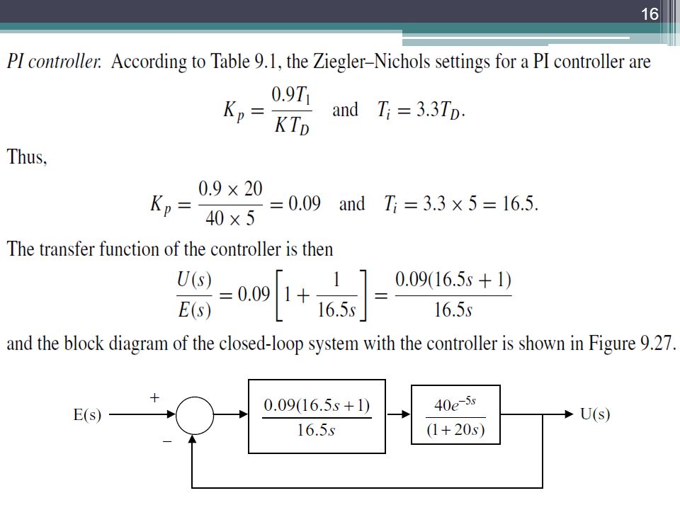
15. The transfer function of the controller is then
and the block diagram of the closed-loop system with the controller is shown below.