Download presentation
Presentation is loading. Please wait.

1
Transmission Lines Dr. Sandra Cruz-Pol ECE Dept. UPRM

2
Exercise 11.3 A 40-m long TL has V g =15 V rms, Z o =30+j60 , and V L =5e -j48 o V rms. If the line is matched to the load and the generator, find: the input impedance Z in, the sending-end current I in and Voltage V in, the propagation constant . Answers: ZLZL ZgZg VgVg + V in - I in +VL-+VL- Z o =30+j60 +j 40 m We’ll solve this problem later, but look at V in and V L At high frequencies, We cannot apply regular circuit theory to electric circuits!

3
Transmission Lines I.TL parameters II.TL Equations III.Input Impedance, SWR, power IV.Smith Chart V.Applications Quarter-wave transformer Slotted line Single stub VI.Microstrips

4
Transmission Lines (TL) TL have two conductors in parallel with a dielectric separating them They transmit TEM waves inside the lines
 TL have two conductors in parallel with a dielectric separating them They transmit TEM waves inside the lines")
5
Common Transmission Lines Two-wire (ribbon) Coaxial Microstrip Stripline (Triplate)
 Coaxial Microstrip Stripline (Triplate)")
6
Other TL (higher order) [Chapter 12]
![Other TL (higher order) [Chapter 12]](http://images.slideplayer.com/24/7427296/slides/slide_6.jpg "Other TL (higher order) [Chapter 12]")
7
Fields inside the TL V proportional to E, I proportional to H

8
Distributed parameters The parameters that characterize the TL are given in terms of per length. R = ohms/meter L = Henries/ m C = Farads/m G = mhos/m

9
Common Transmission Lines R, L, G, and C depend on the particular transmission line structure and the material properties. R, L, G, and C can be calculated using fundamental EMAG techniques. ParameterTwo-Wire LineCoaxial LineParallel-Plate Line Unit R L G C

10
TL representation

11
Distributed line parameters Using KVL:

12
Distributed parameters Taking the limit as z tends to 0 leads to Similarly, applying KCL to the main node gives

13
Wave equation Using phasors The two expressions reduce to Wave Equation for voltage

14
TL Equations Note that these are the wave eq. for voltage and current inside the lines. The propagation constant is and the wavelength and velocity are

15
Transmission Lines I.TL parameters ( R’,L’, G’, C’ ) II.TL Equations ( Z o, …) III.Input Impedance, SWR, power IV.Smith Chart V.Applications Quarter-wave transformer Slotted line Single stub VI.Microstrips
 II.TL Equations ( Z o, …) III.Input Impedance, SWR, power IV.Smith Chart V.Applications Quarter-wave transformer Slotted line Single stub VI.Microstrips")
16
Waves moves through line The general solution is In time domain is Similarly for current, I z

17
Characteristic Impedance of a Line, Z o Is the ratio of positively traveling voltage wave to current wave at any point on the line z

18
Example: An air filled planar line with w =30cm, d =1.2cm, t=3mm, c =7x10 7 S/m. Find R, L, C, G for 500MHz Answer See next w d

19
Common Transmission Lines R, L, G, and C depend on the particular transmission line structure and the material properties. R, L, G, and C can be calculated using fundamental EMAG techniques. ParameterTwo-Wire LineCoaxial LineParallel-Plate Line Unit R L G C

20
Exercise 11.1 A transmission line operating at 500MHz has Z o =80 , =0.04Np/m, =1.5rad/m. Find the line parameters R,L,G, and C. Answer: 3.2 /m, 38.2nH/m, 0.0005 S/m, 5.97 pF/m

21
Different cases of TL Lossless Distortionless Lossy Transmission line

22
Lossless Lines (R=0=G) Has perfect conductors and perfect dielectric medium between them. Propagation: Velocity: Impedance

23
Distortionless line (R/L = G/C) Is one in which the attenuation is independent on frequency. Propagation: Velocity: Impedance

24
Summary j ZoZo General Lossless (R=0=G) Distortionless RC = GL
 Distortionless RC = GL")
25
Excersice 11.2 A telephone line has R=30 /km, L=100 mH/km, G=0, and C= 20 F/km. At 1kHz, obtain: the characteristic impedance of the line, the propagation constant, the phase velocity. Is this a distortionless line? Solution:

26
Transmission Lines I.TL parameters II.TL Equations III.Input Impedance, SWR, power ( Z in, s, P ave ) IV.Smith Chart V.Applications Quarter-wave transformer Slotted line Single stub VI.Microstrips
 IV.Smith Chart V.Applications Quarter-wave transformer Slotted line Single stub VI.Microstrips")
27
Define reflection coefficient at the load, L

28
Terminated TL Then, Similarly, The impedance anywhere along the line is given by The impedance at the load end, Z L, is given by

29
Terminated, Lossless TL Then, Conclusion: The reflection coefficient is a function of the load impedance and the characteristic impedance. Recall for the lossless case, Then

30
Terminated, Lossless TL It is customary to change to a new coordinate system, z = - l, at this point. Rewriting the expressions for voltage and current, we have Rearranging, -z-z z = - l

31
The impedance anywhere along the line is given by The reflection coefficient can be modified as follows Then, the impedance can be written as After some algebra, an alternative expression for the impedance is given by Conclusion: The load impedance is “transformed” as we move away from the load. Impedance (Lossless line)
.")
32
The impedance anywhere along the line is given by The reflection coefficient can be modified as follows Then, the impedance can be written as After some algebra, an alternative expression for the impedance is given by Conclusion: For Lossy TL we use hyperbolic tangent Impedance (Lossy line)
")
33
Exercise : using formulas A 2cm lossless TL has V g =10 V rms, Z g =60 , Z L =100+j80 and Z o =40 , =10cm. Find: the input impedance Z in, the sending-end Voltage V in, ZLZL ZgZg VgVg + V in - I in +VL-+VL- Z o j 2 cm Voltage Divider:

34
Anuncios de actividades Pizza y Pelicula Mar 6 @6pm MissRepresentation Limpieza cascada Gozalandia Mar 9 @7am Earth Hour Mar 29 @ Vieques Ver cortos, info, registro, etc. en http://uprm.edu/eventosverdes

35
Example A generator with 10V rms and R g =50 , is connected to a 75 load thru a 0.8 50 -lossless line. Find V L

36
Transmission Lines I.TL parameters II.TL Equations III.Input Impedance, SWR, power IV.Smith Chart V.Applications Quarter-wave transformer Slotted line Single stub VI.Microstrips

37
SWR or VSWR or s Whenever there is a reflected wave, a standing wave will form out of the combination of incident and reflected waves. (Voltage) Standing Wave Ratio – SWR=VSWR= s is defined as:
 Standing Wave Ratio – SWR=VSWR= s is defined as:.")
38
Transmission Lines I.TL parameters II.TL Equations III.Input Impedance, SWR, power IV.Smith Chart V.Applications Quarter-wave transformer Slotted line Single stub VI.Microstrips

39
Power The average input power at a distance l from the load is given by which can be reduced to The first term is the incident power and the second is the reflected power. Maximum power is delivered to load if =0

40
Three Common Cases of line-load combinations: Shorted Line ( Z L =0 ) Open-circuited Line ( Z L =∞ ) Matched Line ( Z L = Z o )
 Open-circuited Line ( Z L =∞ ) Matched Line ( Z L = Z o )")
41
Standing Waves -Short Shorted Line ( Z L =0 ), we had So substituting in V(z) -z /4 /2 |V(z)| Voltage maxima *Voltage minima occurs at same place that impedance has a minimum on the line
, we had So substituting in V(z) -z /4 /2 |V(z)| Voltage maxima *Voltage minima occurs at same place that impedance has a minimum on the line")
42
Standing Waves -Open Open Line ( Z L =∞ ),we had So substituting in V(z) |V(z)| -z /4 /2 Voltage minima
,we had So substituting in V(z) |V(z)| -z /4 /2 Voltage minima")
43
Standing Waves -Matched Matched Line ( Z L = Z o ), we had So substituting in V(z) |V(z)| -z /4 /2
, we had So substituting in V(z) |V(z)| -z /4 /2 ")
44
Java applets http://www.amanogawa.com/transmission. html http://www.amanogawa.com/transmission. html http://physics.usask.ca/~hirose/ep225/ http://www.home.agilent.com/agilent/applic ation.jspx?nid=- 34943.0.00&cc=PR&lc=eng http://www.home.agilent.com/agilent/applic ation.jspx?nid=- 34943.0.00&cc=PR&lc=eng

45
Transmission Lines I.TL parameters II.TL Equations III.Input Impedance, SWR, power IV.Smith Chart V.Applications Slotted line Quarter-wave transformer Single stub VI.Microstrips

46
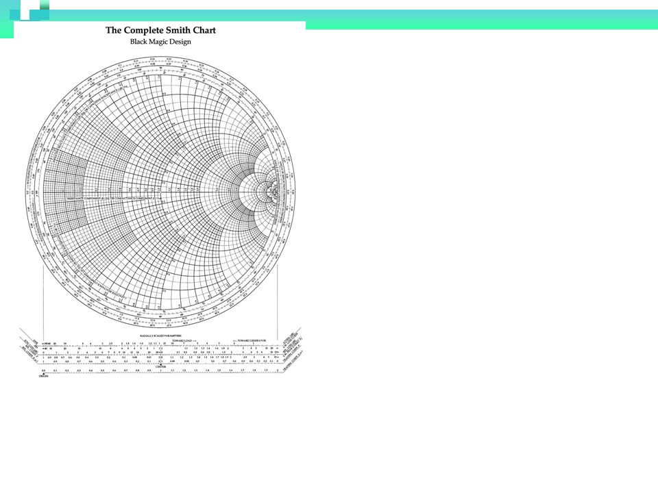
The Smith Chart

47
Smith Chart Commonly used as graphical representation of a TL. Used in hi-tech equipment for design and testing of microwave circuits One turn (360 o ) around the SC = to /2
 around the SC = to /2.")
48
What can be seen on the screen? Network Analyzer

49
Smith Chart Suppose you use as coordinates the reflection coefficient real and imaginary parts. and define the normalized Z L : ii rr

50
Now relating to z=r+jx After some algebra, we obtain two eqs. Similar to general Equation of a Circle of radius a, center at (x,y)= h,k) Circles of r Circles of x
= h,k) Circles of r Circles of x.")
51
Examples of Circles of r and x Circles of r Circles of x

52
Examples of circles of r and x Circles of r Circles of x rr ii

53
Fun facts about the Smith Chart A lossless TL is represented as a circle of constant radius, | |, or constant s Moving along the line from the load toward the generator, the phase decrease, therefore, in the SC equals to moves clockwisely. To generator

54
The joy of the SC Numerically s = r on the +axis of r in the SC Proof:

55
Fun facts about the Smith Chart One turn (360 o ) around the SC = to /2 because in the formula below, if you substitute length for half-wavelength, the phase changes by 2 , which is one turn. Find the point in the SC where =+1,-1, j, -j, 0, 0.5 What is r and x for each case?

56
Fun facts : Admittance in the SC The admittance, y=Y L /Y o where Y o =1/Z o, can be found by moving ½ turn ( /4) on the TL circle
 on the TL circle")
57
Fun facts about the Smith Chart The r +axis, where r > 0 corresponds to V max The r -axis, where r < 0 corresponds to V min V max (Maximum impedance) V min
 V min")
58
Exercise: using S.C. A 2cm lossless TL has V g =10 V rms, Z g =60 , Z L =100+j80 and Z o =40 , =10cm. find: the input impedance Z in, the sending-end Voltage V in, Load is at.2179 @ S.C. Move.2 and arrive to.4179 Read ZLZL ZgZg VgVg + V in - I in +VL-+VL- Z o j 2 cm Voltage Divider:

59
zLzL z in 0.2 towards generator.2179.4179 V min V max

60
Exercise: cont….using S.C. A 2cm lossless TL has V g =10 V rms, Z g =60 , Z L =100+j80 and Z o =40 , =10cm. find: the input impedance Z in, the sending-end Voltage V in, Distance from the load (.2179 to the nearest minimum & max Move to horizontal axis toward the generator and arrive to.5 V max and to.25 for the V min.. Distance to 1 st max=.25 -.2179 =.0321 Distance to 1 st min=.5 -.2179 =.282 Distance to 2 st voltage maximum is.282 See drawing ZLZL ZgZg VgVg + V in - I in +VL-+VL- Z o j 2 cm

61
Exercise : using formulas A 2cm lossless TL has V g =10 V rms, Z g =60 , Z L =100+j80 and Z o =40 , =10cm. find: the input impedance Z in, the sending-end Voltage V in, ZLZL ZgZg VgVg + V in - I in +VL-+VL- Z o j 2 cm Voltage Divider:

62
Another example: A 26cm lossless TL is connected to load Z L =36-j44 and Z o =100 , =10cm. find: the input impedance Z in Load is at.427 @ S.C. Move.1 and arrive to.527 Read ZLZL ZgZg VgVg + V in - I in +VL-+VL- Z o j 26cm Distance to first V max :

63
Exercise 11.4 A 70 lossless line has s =1.6 and =300 o. If the line is 0.6 long, obtain , Z L, Z in and the distance of the first minimum voltage from the load. Answer The load is located at: Move to.4338 and draw line from center to this place, then read where it crosses you TL circle. Distance to V min in this case, l min =.5 -.3338 =

66
Java Applet : Smith Chart http://education.tm.agilent.com/index.cgi?CONTENT_ID=5

67
Transmission Lines I.TL parameters II.TL Equations III.Input Impedance, SWR, power IV.Smith Chart V.Applications Slotted line Quarter-wave transformer Single stub VI.Microstrips

68
Slotted Line Used to measure frequency and load impedance HP Network Analyzer in Standing Wave Display http://www.ee.olemiss.edu/softw are/naswave/Stdwave.pdf

69
Slotted line example Given s, the distance between adjacent minima, and l min for an “air” 100 transmission line, Find f and Z L s=2.4, l min =1.5 cm, l min-min =1.75 cm Solution: =8.6GHz Draw a circle on r=2.4, that’s your T.L. move from V min to z L

70
Transmission Lines I.TL parameters II.TL Equations III.Input Impedance, SWR, power IV.Smith Chart V.Applications Slotted line Quarter-wave transformer Single stub VI.Microstrips

71
Quarter-wave transformer …for impedance matching ZLZL Z in Z o, l= /4 Conclusion: **A piece of line of /4 can be used to change the impedance to a desired value (e.g. for impedance matching)
.")
72
Applications Slotted line as a frequency meter Impedance Matching If Z L is Real: Quarter-wave Transformer ( /4 X mer ) If Z L is complex: Single-stub tuning (use admittance Y)
 If Z L is complex: Single-stub tuning (use admittance Y)")
73
Transmission Lines I.TL parameters II.TL Equations III.Input Impedance, SWR, power IV.Smith Chart V.Applications Quarter-wave transformer Slotted line Single stub VI.Microstrips

74
Single Stub Tuning …for impedance matching A stub is connected in parallel to sum the admittances Use a reactance (Y) from a short-circuited stub or open-circuited stub to cancel reactive part When matched: Z in =Z o therefore z =1 or y=1 (this is our goal!)
 from a short-circuited stub or open-circuited stub to cancel reactive part When matched: Z in =Z o therefore z =1 or y=1 (this is our goal!)")
75
Single Stub Basics We work with Y, because in parallel connections, they add. Y L (=1/Z L ) is to be matched to a TL having characteristic admittance Y o by means of a "stub" consisting of a shorted (or open) section of line having the same characteristic admittance Y o http://web.mit.edu/6.013_book/www/chapter14/14.6.html
 is to be matched to a TL having characteristic admittance Y o by means of a stub consisting of a shorted (or open) section of line having the same characteristic admittance Y o")
76
Single Stub Steps First, the length l is adjusted so that the real part of the admittance at the position where the stub is connected is equal to Y o or y line = 1+ jb Then the length of the shorted stub is adjusted so that it's susceptance cancels that of the line, or y stub = - jb

77
Example: Single Stub A 75 lossless line is to be matched to a 100-j80 load with a shorted stub. Calculate the distance from the load, the stub length, and the necessary stub admittance. Answer: Change z L to admitance : Find d=distance to circle with real=1 as: d=.4338-.3393=0.094 or (both yield same d) Read (1+jb j [or next intersection i.e. 1-jb :d=0.272,] Short stub:.25 -.124 = 0.126 Or 0.376.25 = 0.126 (both yield same distance) With y stub = -j.96/75 * j mhos *[Note que para denormalizar admitancia se divide entre Z o ].4338.3393.0662.1607.124.376
 Read (1+jb j [or next intersection i.e. 1-jb :d=0.272,] Short stub: = Or 0.376.25 = (both yield same distance) With y stub = -j.96/75 * j mhos *[Note que para denormalizar admitancia se divide entre Z o ]")
79
Transmission Lines I.TL parameters II.TL Equations III.Input Impedance, SWR, power IV.Smith Chart V.Applications Quarter-wave transformer Slotted line Single stub VI.Microstrips

80
Microstrips

81
Microstrips analysis equations & Pattern of EM fields

82
Microstrip Design Equations Falta un radical en eff

83
Microstrip Design Curves

84
Example A microstrip with fused quartz ( r =3.8) as a substrate, and ratio of line width to substrate thickness is w/h =0.8, find: Effective relative permittivity of substrate Characteristic impedance of line Wavelength of the line at 10GHz Answer: eff =2.75, Z o =86.03 , =18.09 mm
 as a substrate, and ratio of line width to substrate thickness is w/h =0.8, find: Effective relative permittivity of substrate Characteristic impedance of line Wavelength of the line at 10GHz Answer: eff =2.75, Z o =86.03 , =18.09 mm")
85
Diseño de microcinta: Dado ( r =4) para el substrato, y h =1mm halla w para Z o =30 y cuánto es eff ? Solución: Suponga que como Z es pequeña w/h>2

Similar presentations


 ECE 3317 1 Spring 2014.>")