1. UNIVERSITI MALAYSIA PERLIS
EKT 241/4: ELECTROMAGNETIC THEORY
UNIVERSITI MALAYSIA PERLIS
CHAPTER 5 – TRANSMISSION LINES
PREPARED BY: Saidatul Norlyana Azemi

2. Chapter Outline General Considerations Lumped-Element Model
Transmission-Line Equations
Wave Propagation on a Transmission Line
The Lossless Transmission Line
Input Impedance of the Lossless Line
Special Cases of the Lossless Line
Power Flow on a Lossless Transmission Line
The Smith Chart
Impedance Matching
Transients on Transmission Lines

3. General Considerations
Transmission line – a two-port network connecting a generator circuit to a load.

4. So…What is the use of transmission line??
A transmission line is used to transmit electrical energy/signals from one point to another
i.e. from one source to a load.
Types of transmission line include: wires, (telephone wire), coaxial cables, optical fibers n etc…

5. frequency, f of the signal provided by generator.
The role of wavelength
length of line, l
The impact of a transmission line on the current and voltage in the circuit depends on the:
At low frequency, the impact is negligible
At high frequency, the impact is very significant
frequency, f of the signal provided by generator.

6. Propagation modes Propagation modes Higher order transmission lines
Electric field lines
Propagation modes
Transverse electromagnetic (TEM) transmission lines
waves propagating along these lines having electric and magnetic field that are entirely transverse to the direction of propagation
Higher order transmission lines
waves propagating along these lines have at least one significant field component in the direction of propagation
Magnetic field lines

7. Propagation modes
A few examples of transverse electromagnetic (TEM) and higher order transmission line

8. Lumped- element model
A transmission line is represented by a parallel-wire configuration regardless of the specific shape of the line, (in term of lumped element circuit model)
i.e coaxial line, two-wire line or any TEM line.
Lumped element circuit model consists of four basic elements called ‘the transmission line parameters’ : R’ , L’ , G’ , C’ .
Series element
Shunt element

9. Lumped- element model
Lumped-element transmission line parameters:
R’ : combined resistance of both conductors per unit length, in Ω/m
L’ : the combined inductance of both conductors per unit length, in H/m
G’ : the conductance of the insulation medium per unit length, in S/m
C’ : the capacitance of the two conductors per unit length, in F/m
For example, a coil of wire has the property of inductance. When a certain amount of inductance is needed in a circuit, a coil of the proper dimension is inserted

10. Lumped- element model

11. Lumped- element model for 3 type of lines
Note: µ, σ, ε pertain to the insulating material between conductors

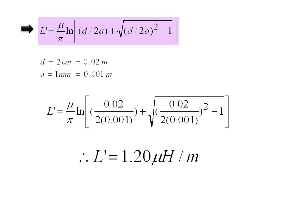
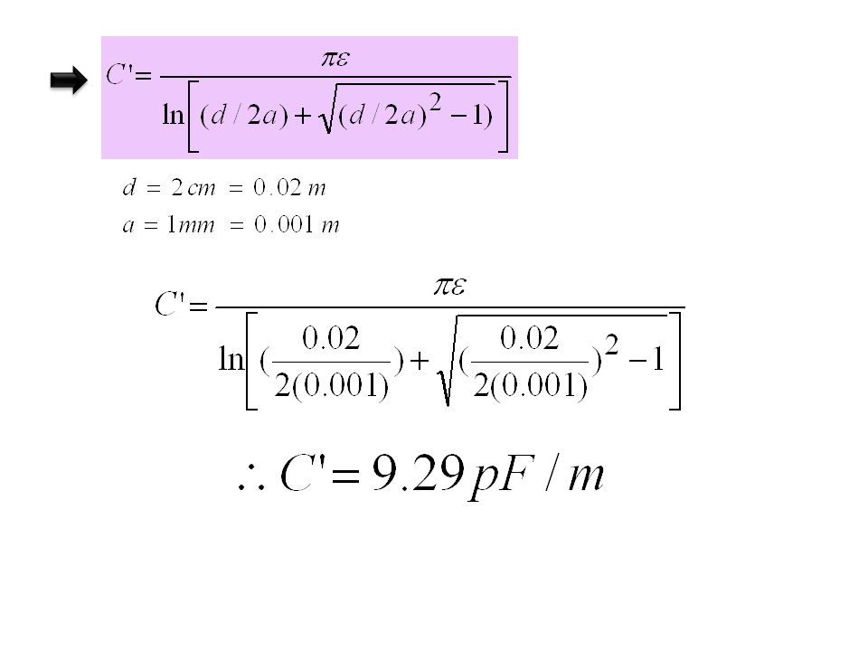
12. Exercise 1:
Use table 5.1 to compute the line parameter of a two wire air line whose wires are separated by distance of 2 cm, and, each is 1 mm in radius. The wires may be treated as perfect conductors with σc= .
R’ = ?, L’=?, G’=?, C’=?

13. Solution exercise 1:
σc= 
σc= 

16. Exercise 2:
Calculate the transmission line parameters at 1 MHz for a rigid coaxial air line with an inner conductor diameter of 0.6 cm and outer conductor diameter of 1.2 cm. The conductors are made of copper.
(μc=0.9991 ; σc=5.8x107)
f = 1MHz
r1 = 0.006m/2 = 0.003m
r2 = 0.012m/2 = 0.006m

17. Solution exercise 2:

18. BARE IN UR MIND
From calculator

19. BARE IN UR MIND
From calculator

20. Because, the material separating the inner and outer is perfect dielectric (air) with σ=0, thus G’ = 0
G’ : the conductance of the insulation medium per unit length, in S/m

21. Transmission line equations
Is used to describes the voltage and the current across the transmission line in term of propagation constant and impedance
Complex propagation constant, γ
α – the real part of γ
- attenuation constant, unit: Np/m
β – the imaginary part of γ
- phase constant, unit: rad/m

22. Transmission line equations
The characteristic impedance of the line, Z0 :
Phase velocity of propagating waves:
where f = frequency (Hz)
λ = wavelength (m)
β = phase constant

23. Example 1
An air line is a transmission line for which air is the dielectric material present between the two conductors, which renders G’ = 0.
In addition, the conductors are made of a material with high conductivity so that R’ ≈0.
For an air line with characteristic impedance of 50Ω and phase constant of 20 rad/m at 700MHz, find the inductance per meter and the capacitance per meter of the line.

24. Solution to Example 1 The following quantities are given:
With R’ = G’ = 0,

25. Solution to Example 1 2
The ratio is given by:
We get L’ from Z0

26. Lossless transmission line
Transmission line can be designed to minimize ohmic losses by selecting high conductivities and dielectric material, thus we assume :
Lossless transmission line - Very small values of R’ and G’.
We set R’=0 and G’=0, hence:

27. Transmission line equations
Complex propagation constant, γ
α – the real part of γ
- attenuation constant, unit: Np/m
β – the imaginary part of γ
- phase constant, unit: rad/m

28. Lossless transmission line
Transmission line can be designed to minimize ohmic losses by selecting high conductivities and dielectric material, thus we assume :
Lossless transmission line - Very small values of R’ and G’.
We set R’=0 and G’=0, hence:

29. Lossless transmission line
Using the relation properties between μ, σ, ε :
Wavelength, λ
Where εr = relative permittivity of the insulating material between conductors

30. Exercise 3:
For a losses transmission line, λ = 20.7 cm at 1GHz. Find εr of the insulating material.
λ=20.7cm 0.207m ; f=1 GHz 2

31. Exercise 4
A lossless transmission line of length 80 cm operates at a frequency of . The line parameters are & Find the characteristic impedance, the phase constant and the phase velocity.
The condition apply that the line is lossless, So: R= 0 & G=0

32. characteristic impedance :
phase constant:
With R n G = 0
= rad/m

33. phase velocity:

34. Voltage Reflection Coefficient
Every transmission line has a resistance associated with it, and comes about because of its construction. This is called its characteristic impedance, Z0.
The standard characteristic impedance value is 50Ω. However when the transmission line is terminated with an arbitrary load ZL, in which is not equivalent to its characteristic impedance (ZL ≠ Z0), a reflected wave will occur.

35. Voltage reflection coefficient
Voltage reflection coefficient, Γ – the ratio of the amplitude of the reflected voltage wave, V0- to the amplitude of the incident voltage wave, V0+ at the load.
Hence,

36. Voltage reflection coefficient
The load impedance, ZL
Where;
= total voltage at the load
V0- = amplitude of reflected voltage wave
V0+ = amplitude of the incident voltage wave
= total current at the load
Z0 = characteristic impedance of the line

37. Voltage reflection coefficient
And in case of a RL and RC series, ZL :
ZL = R + jL ; ZL = R -1/ jC
A load is matched to the line if ZL = Z0 because there will be no reflection by the load (Γ = 0 and V0−= 0.
When the load is an open circuit, (ZL=∞), Γ = 1 and V0- = V0+.
When the load is a short circuit (ZL=0), Γ = -1 and V0- = V0+.

38. What is the difference between an open and closed circuit?
closed allows electricity through, and open doesn't.
open circuit - Any circuit which is not complete is considered an open circuit. The open status of the circuit doesn't depend on how it became unclosed, so circuits which are manually disconnected and circuits which have blown fuses, faulty wiring or missing components are all considered open circuits.
close circuit: A circuit is considered to be closed when electricity flows from an energy source to the desired endpoint of the circuit. A complete circuit which is not performing any actual work can still be a closed circuit. For example, a circuit connected to a dead battery may not perform any work, but it is still a closed circuit.

39. Example 2
A 100-Ω transmission line is connected to a load consisting of a 50-Ω resistor in series with a 10pF capacitor. Find the reflection coefficient at the load for a 100-MHz signal.

40. Solution to Example 2 The following quantities are given
The load impedance is
Voltage reflection coefficient is

41. In order to convert from –ve magnitude for Г by replacing the –ve sign with e-j180

42. Math’s TIP… 1 2

43. Exercise 5
A 150 Ω lossless line is terminated in a load impedance ZL= (30 –j200) Ω. Calculate the voltage reflection coefficient at the load.
Zo = 150 Ω
ZL= (30 –j200) Ω

44. Standing Waves
Interference of the reflected wave and the incident wave along a transmission line creates a standing wave.
Constructive interference gives maximum value for standing wave pattern, while destructive interference gives minimum value.
The repetition period is λ for incident and reflected wave individually.
But, the repetition period for standing wave pattern is λ/2.

45. Standing Waves For a matched line, ZL = Z0, Γ = 0 and
= |V0+| for all values of z.

46. Standing Waves
For a short-circuited load, (ZL=0), Γ = -1.

47. Standing Waves For an open-circuited load, (ZL=∞), Γ = 1.
The wave is shifted by λ/4 from short-circuit case.

48. Standing Waves First voltage maximum occurs at: If θr ≥ 0  n=0;
First voltage minimum occurs at:
Where θr = phase angle of Γ

49. VSWR The VSWR is given by:
Voltage Standing Wave Ratio (VSWR) is ratio between the maximum voltage an the minimum voltage along the transmission line.
VSWR provides a measure of mismatch between the load and the transmission line.
For a matched load with Γ = 0, VSWR = 1 and for a line with |Γ| - 1, VSWR = ∞.
The VSWR is given by:

50. Example 3
A 50- transmission line is terminated in a load with ZL = (100 + j50)Ω . Find the voltage reflection coefficient and the voltage standing-wave ratio (VSWR).

51. Solution to Example 3
We have,
VSWR is given by:

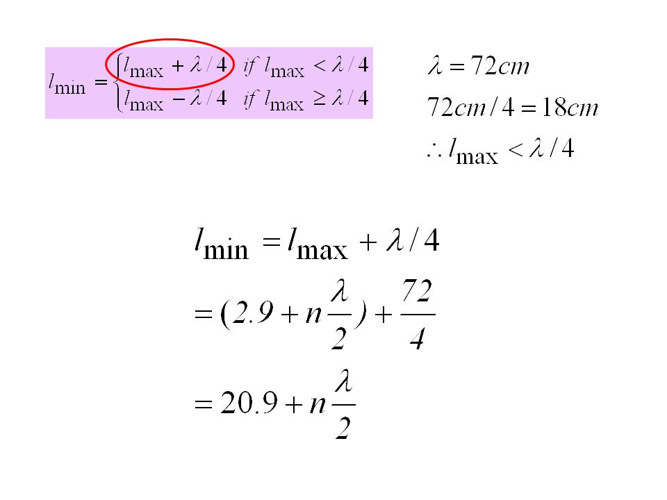
52. Exercise 6:
A 140 Ω lossless line is terminated in a load impedance ZL= (280 +j182) Ω, if λ = 72cm, find
a) Reflection coefficient, Г
b) The VSWR,
c) The locations of voltage maxima and minima

53. a) Reflection coefficient, Г

54. b) The VSWR;

55. The locations of voltage maxima and minima

57. Input impedance of a lossless line
The input impedance, Zin is the ratio of the total voltage (incident and reflected voltages) to the total current at any point z on the line. or

58. Special cases of the lossless line
For a line terminated in a short-circuit, ZL = 0:
For a line terminated in an open circuit, ZL = ∞:

59. Application of short-circuit and open-circuit measurements
The measurements of short-circuit input impedance, and open-circuit input impedance, can be used to measure the characteristic impedance of the line:
and

60. Length of line
If the transmission line has length , where n is an integer,
Hence, the input impedance becomes:

61. Quarter wave transformer
If the transmission line is a quarter wavelength, with , where , we have , then the input impedance becomes:

62. Example 4
A 50-Ω lossless transmission line is to be matched to a resistive load impedance with ZL=100Ω via a quarter-wave section as shown, thereby eliminating reflections along the feedline. Find the characteristic impedance of the quarter-wave transformer.

63. Quarter wave transformer
If the transmission line is a quarter wavelength, with , where , we have , then the input impedance becomes:

64. Solution to Example 4 Zin = 50Ω; ZL=100Ω
Since the lines are lossless, all the incident power will end up getting transferred into the load ZL.

65. Matched transmission line
For a matched lossless transmission line, ZL=Z0:
1) The input impedance Zin=Z0 for all locations z on the line,
2) Γ =0, and
3) all the incident power is delivered to the load, regardless of the length of the line, l.

66. Input Impedance, Zin When ZL=0(short circuit)
Ratio of the total voltage to total current on the line
Special case
When ZL=(open circuit)
Input Impedance, Zin
Application
Be used to measure the characteristic impedance of the line :
But, If the transmission line is

67. Power flow on a lossless transmission line
Two ways to determine the average power of an incident wave and the reflected wave;
Time-domain approach
Phasor domain approach
Average power for incident wave;
Average power for reflected wave:
The net average power delivered to the load:

68. Power flow on a lossless transmission line
The time average power reflected by a load connected to a lossless transmission line is equal to the incident power multiplied by |Г|2

69. Exercise 7
For a 50Ω lossless transmission line terminated in a load impedance ZL = (100 + j50)Ω, determine the percentage of the average power reflected over average incident power by the load.
Z0=50Ω; ZL = (100 + j50)Ω

70. Reflection coefficient, Г
the percentage of the average incident power reflected by the load = 20%

71. Exercise 8
For the line of exercise previously (exercise 7), what is the average reflected power if |V0+|=1V

72. Гr = real part, Гi = imaginary part
Smith Chart
Smith chart is used to analyze & design transmission line circuits.
Reflection coefficient, Γ :
Гr = real part, Гi = imaginary part
Impedances on Smith chart are represented by normalized value, zL :
the normalized load impedance, zL is dimensionless.

73. Smith Chart Reflection coefficient, ΓA :0.3 + j0.4
Reflection coefficient, ΓB : j0.2
In order to eliminate –ve part, thus

74. The complex Γ plane.
ΓA :0.3 + j0.4
ΓB : j0.2

75. Smith Chart Reflection coefficient, Γ : Since , Γ becomes:
Re-arrange in terms of zL:
rL = Normalized load resistance
xL = Normalized load admittance

76. The families of circle for rL and xL.

77. Plotting normalized impedance, zL = 2-j1

78. Input impedance The input impedance, Zin:
Γ is the voltage reflection coefficient at the load.
We shift the phase angle of Γ by 2βl, to get ΓL. This will zL to zin. The |Γ| is the same, but the phase is changed by 2βl.
On the Smith chart, this means rotating in a clockwise direction (WTG).

79. Input impedance
Since β = 2π/λ, shifting by 2 βl is equal to phase change of 2π.
Equating:
Hence, for one complete rotation corresponds to l = λ/2.
The objective of shifting Γ to ΓL is to find Zin at an any distance l on the transmission line.

80. Example 5
A 50-Ω transmission line is terminated with ZL=(100-j50)Ω. Find Zin at a distance l =0.1λ from the load.
Solution:
Normalized the load impedance

81. de normalize (multiplying by Zo) Zin = 30 –j33
Solution to Example 5
l =0.1λ
zin = 0.6 –j0.66
de normalize (multiplying by Zo) Zin = 30 –j33

82. VSWR, Voltage Maxima and Voltage Minima
zL=2+j1
VSWR = 2.6
(at Pmax).
lmax=( )λ
=0.037λ.
lmin=( )λ
=0.287λ

83. VSWR, Voltage Maxima and Voltage Minima
Point A is the normalized load impedance with zL=2+j1.
VSWR = 2.6 (at Pmax).
The distance between the load and the first voltage maximum is lmax=( )λ=0.037λ.
The distance between the load and the first voltage minimum is lmin=( )λ =0.287λ.

84. Impedance to admittance transformations
zL=0.6 + j1.4
yL= j0.6

85. Example 6
Given that the voltage standing-wave ratio, VSWR = 3. On a 50-Ω line, the first voltage minimum occurs at 5 cm from the load, and that the distance between successive minima is 20 cm, find the load impedance.
Solution:
The distance between successive minima is equal to λ/2.
the distance between successive minima is 20 cm, Hence, λ = 40 cm

86. de normalize (multiplying by Zo) Zin = 30 –j40
Solution to Example 6
Point A =VSWR = 3
de normalize (multiplying by Zo) Zin = 30 –j40

87. Solution to Example 6 First voltage minimum (in wavelength unit) is at
on the WTL scale from point B.
Intersect the line with constant SWR circle = 3.
The normalized load impedance at point C is:
De-normalize (multiplying by Z0) to get ZL:

88. Exercise

89. Solution:
Normalized the load impedance
a) reflection coefficient from smith Chart

90. lmax
lmin

91. Move a distance 0.301λ towards the generator (WTG) (refer to Smith chart) 
→ 0.301λ λ=0.383λ
At 0.383λ, read the value of which at the point intersects with constant circle, we have = zin = j0.62.
Denormalized it, hence = Zin = 72- j62
Distance from load to the first voltage maximum, (refer to Smith chart)
→ 0.25λ-0.082λ=0.168λ

92. Impedance Matching
Transmission line is matched to the load when Z0 = ZL.
This is usually not possible since ZL is used to serve other application.
Alternatively, we can place an impedance-matching network between load and transmission line.

93. Single- stub matching
Matching network consists of two sections of transmission lines.
First section of length d, while the second section of length l in parallel with the first section, hence it is called stub.
The second section is terminated with either short-circuit or open circuit.

94. Single- stub matching
YL=1/ZL
stub l
feed line d
Yd = Y0+jB

95. Single- stub matching
The length l of the stub is chosen so that its input admittance, YS at MM’ is equal to –jB.
Hence, the parallel sum of the two admittances at MM’ yields Y0, which is the characteristic admittance of the line.
Yd = Y0+jB

96. Single- stub matching
Thus, the main idea of shunt stub matching network is to:
(i) Find length d and l in order to get yd and yl .
(ii) Ensure total admittance yin = yd + ys = 1 for complete matching network.

97. Example 7
50-Ω transmission line is connected to an antenna with load impedance ZL = (25 − j50)Ω. Find the position and length of the short-circuited stub required to match the line.
Solution:
The normalized load impedance is:
(located at A).

98. Solution to Example 7

99. Solution to Example 7
Value of yL at B is which locates at position 0.115λ on the WTG scale.
Draw constant SWR circle that goes through points A and B.
There are two possible matching points, C and D where the constant SWR circle intersects with circle rL=1 (now gL =1 circle).

100. B
C = 1+j1.58
D = 1+j1.58 A

101. Solution to Example 7 First matching points, C.
At C, is at 0.178λ on WTG scale.
Distance B and C is
Normalized input admittance
at the juncture is:
E is the admittance of short-circuit stub, yL=-j∞.
Normalized admittance of −j 1.58 at F and position 0.34λ on the WTG scale gives:

102. d1
= 0.063λ B
C = 1+j1.58 E l1
= 0.090λ A
F = -j1.58 F

103. First matching points, C
Thus, the values are:
d1 = λ
l1 = 0.09 λ
yd1 = 1 + j1.58 Ω
ys1 = -j1.58 Ω
Where Yin = yd + ys = (1 + j1.58) + (-j1.58) = 1

104. Solution to Example 7 Second matching point, D. At point D,
Distance B and D is
Normalized input admittance at G.
Rotating from point E to point G, we get

105. B G
G = +j1.58 d2
= 0.207λ E l2
= 0.41λ
D = 1-j1.58 A

106. First matching points, D
Thus, the values are:
d2 = λ
l2 = 0.41 λ
yd2 = 1 - j1.58 Ω
ys2 = +j1.58 Ω
Where Yin = yd + ys = (1 - j1.58) + (+j1.58) = 1

107. d1=0.063 λ
d2=0.207 λ
l1=0.09λ,
l2=0.41 λ