Download presentation
Presentation is loading. Please wait.

1
Summary of Previous Lecture

2
Summary of Previous Lecture
We covered the following topics in today’s lecture Value creation and the key sources of value creation for the firm. Overall cost of capital of the firm. Costs of the individual components of a firm’s cost of capital - cost of debt, cost of preferred stock, and cost of equity. Alternative models to determine the cost of equity, including the dividend discount approach, the capital-asset pricing model (CAPM) approach, and the before-tax cost of debt plus risk premium approach.
 approach, and the before-tax cost of debt plus risk premium approach.")
3
Required Returns and the Cost of Capital
Chapter 15 (II) Required Returns and the Cost of Capital
 Required Returns and the Cost of Capital.")
4
Learning Outcomes After studying Chapter 15, you should be able to:
Explain how a firm creates value and identify the key sources of value creation. Define the overall “cost of capital” of the firm. Calculate the costs of the individual components of a firm’s cost of capital - cost of debt, cost of preferred stock, and cost of equity. Explain and use alternative models to determine the cost of equity, including the dividend discount approach, the capital-asset pricing model (CAPM) approach, and the before-tax cost of debt plus risk premium approach. Calculate the firm’s weighted average cost of capital (WACC) and understand its rationale, use, and limitations. Explain how the concept of Economic Value Added (EVA) is related to value creation and the firm’s cost of capital. Understand the capital-asset pricing model's role in computing project-specific and group-specific required rates of return.
 approach, and the before-tax cost of debt plus risk premium approach. Calculate the firm’s weighted average cost of capital (WACC) and understand its rationale, use, and limitations. Explain how the concept of Economic Value Added (EVA) is related to value creation and the firm’s cost of capital. Understand the capital-asset pricing model s role in computing project-specific and group-specific required rates of return.")
5
Weighted Average Cost of Capital (WACC)
Cost of Capital = kx(Wx) S n x=1 Amount of financing (1) Proportion of Total Financing (2) Debt $ 30 million 30 % Preferred Stock $ 10 million 10 % Common Stock $ 60 million 60 %
 S. n. x=1. Amount of financing. (1) Proportion of Total Financing (2) Debt. $ 30 million. 30 % Preferred Stock. $ 10 million. 10 % Common Stock. $ 60 million. 60 %")
6
Weighted Average Cost of Capital (WACC)
(1) Cost (2) Proportion of Total Financing X (2) Weighted Cost Debt 6.60 % 30 % 1.98 % Preferred Stock 10.2 % 10 % 1.02 % Common Stock Equity 14.0 % 60 % 8.40 %
 Cost. (2) Proportion of Total Financing. X (2) Weighted Cost. Debt % 30 % 1.98 % Preferred Stock % 10 % 1.02 % Common Stock Equity % 60 % 8.40 %")
7
Limitations of the WACC
1. Weighting System Marginal Capital Costs Capital Raised in Different Proportions than WACC The firm should raise capital marginally in proportion of the capital for the new investments. Real capital cost of newly raised capital will be different because of different proportion of capital raised.

8
Limitations of the WACC
2. Flotation Costs are the costs associated with issuing securities such as underwriting, legal, listing, and printing fees. a. Adjustment to Initial Outlay b. Adjustment to Discount Rate

9
Adjustment to Initial Outlay (AIO)
Add Flotation Costs (FC) to the Initial Cash Outlay (ICO). Impact: Reduces the NPV n CFt NPV = S - ( ICO + FC ) (1 + k)t t=1
 to the Initial Cash Outlay (ICO). Impact: Reduces the NPV. n. CFt. NPV = S. - ( ICO + FC ) (1 + k)t. t=1.")
10
Adjustment to Discount Rate (ADR)
Subtract Flotation Costs from the proceeds (price) of the security and recalculate yield figures. Impact: Increases the cost for any capital component with flotation costs. Result: Increases the WACC, which decreases the NPV.
 of the security and recalculate yield figures. Impact: Increases the cost for any capital component with flotation costs. Result: Increases the WACC, which decreases the NPV.")
11
Economic Value Added Specific measure developed by Stern Stewart and Company in late 1980s. A measure of business performance. It is another way of measuring that firms are earning returns on their invested capital that exceed their cost of capital.

12
Economic Value Added EVA = NOPAT – [Cost of Capital x Capital Employed] Since a cost is charged for equity capital also, a positive EVA generally indicates shareholder value is being created. Based on Economic NOT Accounting Profit. NOPAT – net operating profit after tax is a company’s potential after-tax profit if it was all-equity-financed or “unlevered.”
![Economic Value Added EVA = NOPAT – [Cost of Capital x Capital Employed]](http://slideplayer.com/slide/7107873/24/images/12/Economic+Value+Added+EVA+%3D+NOPAT+%E2%80%93+%5BCost+of+Capital+x+Capital+Employed%5D.jpg "Since a cost is charged for equity capital also, a positive EVA generally indicates shareholder value is being created. Based on Economic NOT Accounting Profit. NOPAT – net operating profit after tax is a company’s potential after-tax profit if it was all-equity-financed or unlevered.")
13
Determining Project-Specific Required Rates of Return
Use of CAPM in Project Selection: Initially assume all-equity financing. Determine project beta. Calculate the expected return. Adjust for capital structure of firm. Compare cost to IRR of project.

14
Difficulty in Determining the Expected Return
Determining the SML: Locate a proxy for the project (much easier if asset is traded). Plot the Characteristic Line relationship between the market portfolio and the proxy asset excess returns. Estimate beta and create the SML.
. Plot the Characteristic Line relationship between the market portfolio and the proxy asset excess returns. Estimate beta and create the SML.")
15
Project Acceptance and/or Rejection
X SML X X X X O X X EXPECTED RATE OF RETURN O O O O Reject O Rf O SYSTEMATIC RISK (Beta)
")
16
Determining Project-Specific Required Rate of Return
1. Calculate the required return for Project k (all-equity financed). Rk = Rf + (Rm - Rf)bk Adjust for capital structure of the firm (financing weights). Weighted Average Required Return = [ki][% of Debt] + [Rk][% of Equity]
. Rk = Rf + (Rm - Rf)bk. Adjust for capital structure of the firm (financing weights). Weighted Average Required Return. = [ki][% of Debt] + [Rk][% of Equity]")
17
Project-Specific Required Rate of Return Example
Assume a computer networking project is being considered with an IRR of 19%. Examination of firms in the networking industry allows us to estimate an all-equity beta of Our firm is financed with 70% Equity and 30% Debt at ki=6%. The expected return on the market is 11.2% and the risk-free rate is 4%.

18
Do You Accept the Project?
ke = Rf + (Rm - Rf)bj = 4% + (11.2% - 4%)1.5 ke = 4% % = 14.8% WACC = .30(6%) + .70(14.8%) = 1.8% % = 12.16% IRR = 19% > WACC = 12.16% If IRR > WACC, then the project is acceptable because it will return a rate of return on invested capital that is likely to be greater than the cost of funds used to invest in the project.
bj. = 4% + (11.2% - 4%)1.5. ke = 4% % = 14.8% WACC = .30(6%) + .70(14.8%) = 1.8% % = 12.16% IRR = 19% > WACC = 12.16% If IRR > WACC, then the project is acceptable because it will return a rate of return on invested capital that is likely to be greater than the cost of funds used to invest in the project.")
19
Determining Group-Specific Required Rates of Return
Use of CAPM in Project Selection: Initially assume all-equity financing. Determine group beta. Calculate the expected return. Adjust for capital structure of group. Compare cost to IRR of group project.

20
Comparing Group-Specific Required Rates of Return
Company Cost of Capital Expected Rate of Return Group-Specific Required Returns Systematic Risk (Beta)
")
21
Qualifications to Using Group-Specific Rates
Amount of non-equity financing relative to the proxy firm. Adjust project beta if necessary. Standard problems in the use of CAPM. Potential insolvency is a total-risk problem rather than just systematic risk (CAPM).
.")
22
Project Evaluation Based on Total Risk
Risk-Adjusted Discount Rate Approach (RADR) The required return is increased (decreased) relative to the firm’s overall cost of capital for projects or groups showing greater (smaller) than “average” risk. Advantages of risk adjusted discount rate It is simple and can be easily understood. It has a great deal of intuitive appeal for risk-averse managers. It incorporates an attitude towards uncertainty.
 The required return is increased (decreased) relative to the firm’s overall cost of capital for projects or groups showing greater (smaller) than average risk. Advantages of risk adjusted discount rate. It is simple and can be easily understood. It has a great deal of intuitive appeal for risk-averse managers. It incorporates an attitude towards uncertainty.")
23
RADR and NPV Adjusting for risk correctly $000s
may influence the ultimate Project decision. $000s 15 10 RADR – “low” risk at 10% (Accept!) Net Present Value 5 RADR – “high” risk at 15% (Reject!) -4 Discount Rate (%)
 Net Present Value. 5. RADR – high risk at 15% (Reject!) Discount Rate (%)")
24
Project Evaluation Based on Total Risk
Probability Distribution Approach Acceptance of a single project with a positive NPV depends on the dispersion of NPVs and the utility preferences of management.

25
Firm-Portfolio Approach
Indifference Curves C B EXPECTED VALUE OF NPV A Curves show “HIGH” Risk Aversion STANDARD DEVIATION

26
Firm-Portfolio Approach
Indifference Curves C B EXPECTED VALUE OF NPV A Curves show “MODERATE” Risk Aversion STANDARD DEVIATION

27
Firm-Portfolio Approach
Indifference Curves B EXPECTED VALUE OF NPV A Curves show “LOW” Risk Aversion STANDARD DEVIATION

28
Adjusting Beta for Financial Leverage
bj = bju [ 1 + (B/S)(1-TC) ] bj: Beta of a levered firm. bju: Beta of an unlevered firm (an all-equity financed firm). B/S: Debt-to-Equity ratio in Market Value terms. TC : The corporate tax rate.
(1-TC) ] bj: Beta of a levered firm. bju: Beta of an unlevered firm (an all-equity financed firm). B/S: Debt-to-Equity ratio in Market Value terms. TC : The corporate tax rate.")
29
Adjusted Present Value
Adjusted Present Value (APV) is the sum of the discounted value of a project’s operating cash flows plus the value of any tax-shield benefits of interest associated with the project’s financing minus any flotation costs. APV = Unlevered Project Value + Value of Project Financing
 is the sum of the discounted value of a project’s operating cash flows plus the value of any tax-shield benefits of interest associated with the project’s financing minus any flotation costs. APV = Unlevered. Project Value. + Value of. Project Financing.")
30
NPV and APV Example Assume AB Corporation is considering a new $425,000 automated machine that will save $100,000 per year for the next 6 years. The required rate on unlevered equity is 11%. ABC can borrow $180,000 at 7% with $10,000 after-tax flotation costs. Principal is repaid at $30,000 per year (+ interest). The firm is in the 40% tax bracket.
. The firm is in the 40% tax bracket.")
31
AB Corporation NPV Solution
What is the NPV to an all-equity-financed firm? NPV = $100,000[PVIFA11%,6] - $425,000 NPV = $423,054 - $425,000 NPV = -$1,946

32
AB Corporation APV Solution
What is the APV? First, determine the interest expense. Int Yr 1 ($180,000)(7%) = $12,600 Int Yr 2 ( 150,000)(7%) = 10,500 Int Yr 3 ( 120,000)(7%) = 8,400 Int Yr 4 ( 90,000)(7%) = 6,300 Int Yr 5 ( 60,000)(7%) = 4,200 Int Yr 6 ( 30,000)(7%) = 2,100
(7%) = $12,600 Int Yr 2 ( 150,000)(7%) = 10,500 Int Yr 3 ( 120,000)(7%) = 8,400 Int Yr 4 ( 90,000)(7%) = 6,300 Int Yr 5 ( 60,000)(7%) = 4,200 Int Yr 6 ( 30,000)(7%) = 2,100.")
33
AB Corporation APV Solution
Second, calculate the tax-shield benefits. TSB Yr 1 ($12,600)(40%) = $5,040 TSB Yr 2 ( 10,500)(40%) = 4,200 TSB Yr 3 ( 8,400)(40%) = 3,360 TSB Yr 4 ( 6,300)(40%) = 2,520 TSB Yr 5 ( 4,200)(40%) = 1,680 TSB Yr 6 ( 2,100)(40%) =
(40%) = $5,040. TSB Yr 2 ( 10,500)(40%) = 4,200. TSB Yr 3 ( 8,400)(40%) = 3,360. TSB Yr 4 ( 6,300)(40%) = 2,520. TSB Yr 5 ( 4,200)(40%) = 1,680. TSB Yr 6 ( 2,100)(40%) = 840.")
34
AB Corporation APV Solution
Third, find the PV of the tax-shield benefits. TSB Yr 1 ($5,040)(.901) = $4,541 TSB Yr 2 ( 4,200)(.812) = 3,410 TSB Yr 3 ( 3,360)(.731) = 2,456 TSB Yr 4 ( 2,520)(.659) = 1,661 TSB Yr 5 ( 1,680)(.593) = TSB Yr 6 ( )(.535) = PV = $13,513
(.901) = $4,541. TSB Yr 2 ( 4,200)(.812) = 3,410. TSB Yr 3 ( 3,360)(.731) = 2,456. TSB Yr 4 ( 2,520)(.659) = 1,661. TSB Yr 5 ( 1,680)(.593) = 996. TSB Yr 6 ( 840)(.535) = 449 PV = $13,513.")
35
AB Corporation NPV Solution
What is the APV? APV = NPV + PV of TS - Flotation Cost APV = -$1,946 + $13,513 - $10,000 APV = $1,567

37
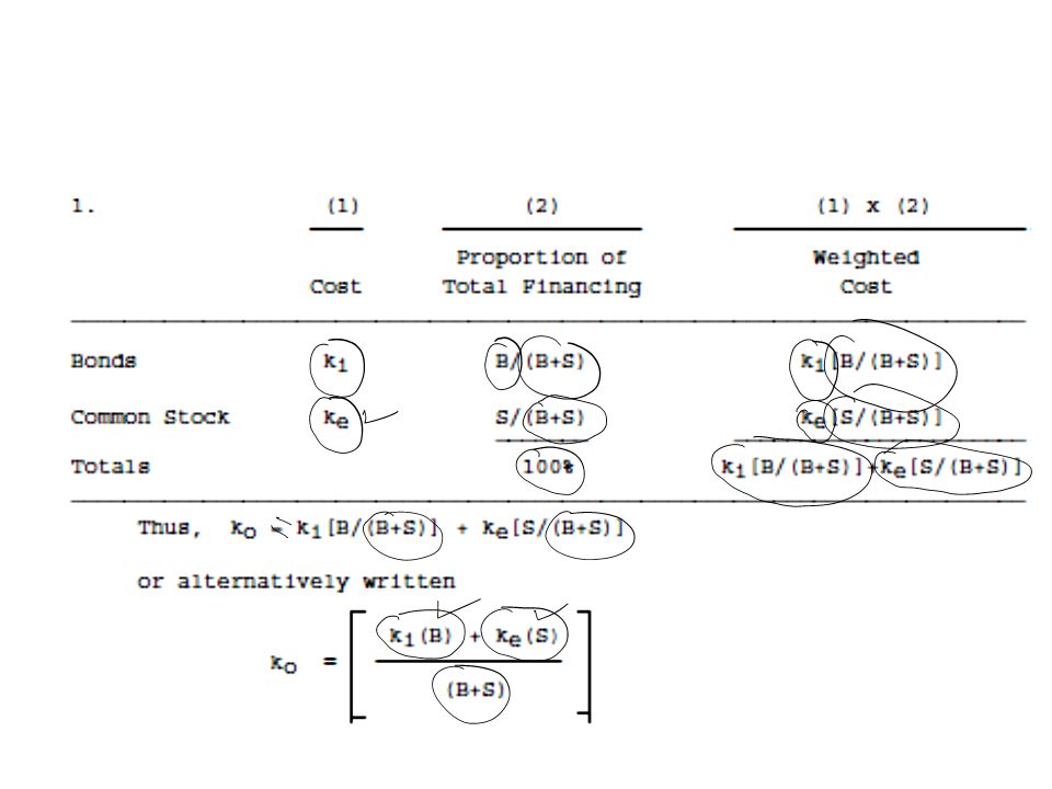
Problem 1 Zapata Enterprises is financed by two sources of funds: bonds and common stock. The cost of capital for funds provided by bonds is ki, and ke is the cost of capital for equity funds. The capital structure consists of B dollars’ worth of bonds and S dollars’ worth of stock, where the amounts represent market values. Compute the overall weighted average of cost of capital, ko.

39
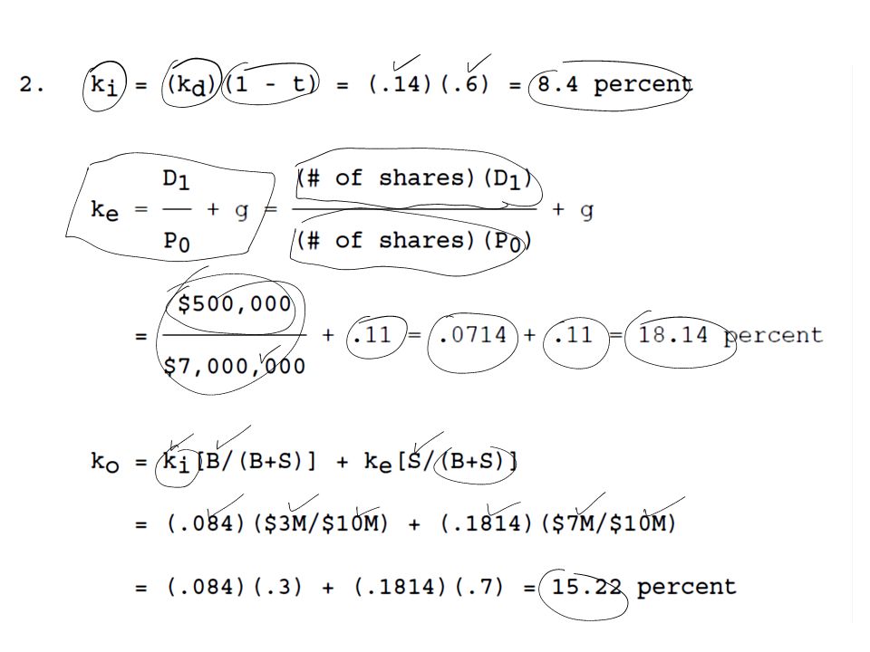
Problem 2 Assume that B (in Problem 1) is $3 million and S is $7 million. The bonds have a 14 percent yield to maturity, and the stock is expected to pay $500,000 in dividends this year. The growth rate of dividends has been 11 percent and is expected to continue at the same rate. Find the cost of capital if the corporation tax rate on income is 40 percent.
 is $3 million and S is $7 million. The bonds have a 14 percent yield to maturity, and the stock is expected to pay $500,000 in dividends this year. The growth rate of dividends has been 11 percent and is expected to continue at the same rate. Find the cost of capital if the corporation tax rate on income is 40 percent.")
41
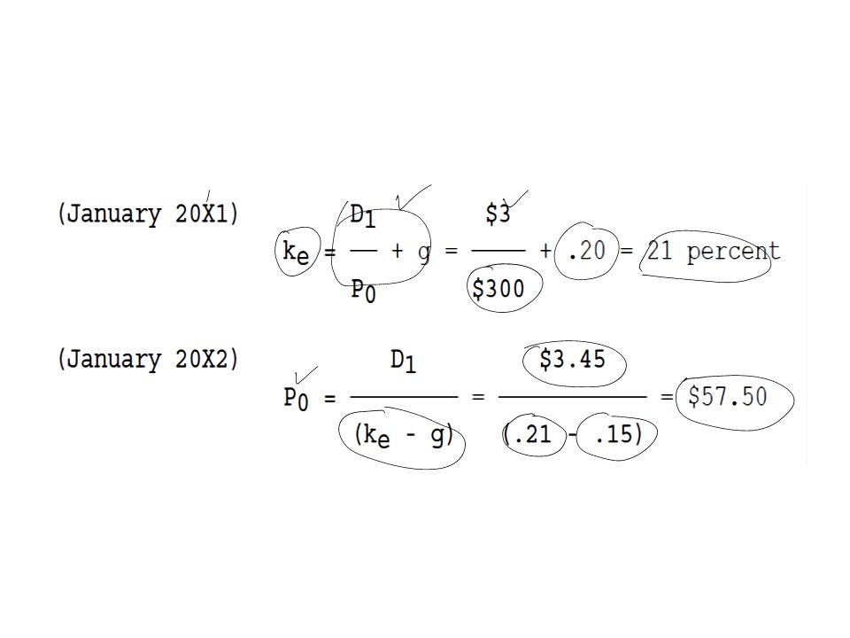
Problem 3 On January 1, 20X1, International Copy Machines (ICOM), one of the favorites of the stock market, was priced at $300 per share. This price was based on an expected dividend at the end of the year of $3 per share and an expected annual growth rate in dividends of 20 percent into the future. By January 20X2, economic indicators have turned down, and investors have revised their estimate for future dividend growth of ICOM downward to 15 percent. What should be the price of the firm’s common stock in January 20X2? Assume the following: a. A constant dividend growth valuation model is a reasonable representation of the way the market values ICOM. b. The firm does not change the risk complexion of its assets nor its financial leverage. c. The expected dividend at the end of 20X2 is $3.45 per share.
, one of the favorites of the stock market, was priced at $300 per share. This price was based on an expected dividend at the end of the year of $3 per share and an expected annual growth rate in dividends of 20 percent into the future. By January 20X2, economic indicators have turned down, and investors have revised their estimate for future dividend growth of ICOM downward to 15 percent. What should be the price of the firm’s common stock in January 20X2 Assume the following: a. A constant dividend growth valuation model is a reasonable representation of the way the market values ICOM. b. The firm does not change the risk complexion of its assets nor its financial leverage. c. The expected dividend at the end of 20X2 is $3.45 per share.")
43
Summary We covered the following topics in today’s lecture;
Firm’s weighted average cost of capital (WACC) and understand its rationale, use, and limitations. Concept of Economic Value Added (EVA) is related to value creation and the firm’s cost of capital. Understand the capital-asset pricing model's role in computing project-specific and group-specific required rates of return.
 and understand its rationale, use, and limitations. Concept of Economic Value Added (EVA) is related to value creation and the firm’s cost of capital. Understand the capital-asset pricing model s role in computing project-specific and group-specific required rates of return.")
Similar presentations