1. Introduction to Image Processing
Filtering in the Frequency Domain
Grass
Sky
Tree ?
Discrete Fourier Transform

2. Image Enhancement in the Frequency Domain
The frequency is the number of oscillations per second. The higher the frequency, the shorter the period. In imaging, it means how quickly/slowly the grey level intensity changes.
Images represent variations of brightness or colour in space. If the variation is spatial and L, the period is a distance, then 1/L is termed the spatial frequency of the variation.
A High Frequency Signal (1-D)
A Low Frequency Signal (1-D)

3. Why Frequency Domain?
The frequency domain describes the rate of signal change. We can associate frequencies in the Fourier Transform with patterns of intensity variations in the image. Thus different information about an image can be extracted and manipulated.
Some tasks would be difficult or impossible to perform directly in the spatial domain, e.g., it is very difficult to do a good job of sharpening a blurred image caused by motion in the spatial domain. This task is generally solved by frequency domain filtering.
Spatial domain filters are useful for lessening the effects of additive/random noise. However in the frequency domain we can uncover patterned noise (e.g. sinusoidal noise) and remove it using band reject/notch frequency domain filters.
Applying the equivalent filters in the spatial domain involves convolution which requires a great amount of computation

4. Fourier Theory Basic ideas:
A periodic function, however complex it might appear, can be represented as a weighted sum of sines/cosines functions of different frequencies.
Although there may be little regularity apparent in an image, it can be decomposed into a set of sinusoidal components, each of which has a well defined frequency.

5. Fourier transform basis functions
Example 1
Fourier transform basis functions
Approximating a square wave as the sum of sine waves

6. Example 2 time domain frequency domain
Another familiar example is sun glasses with UV filter which removes the ultra-violet - very high frequency - component from the sunshine.

7. Fourier Transform 1-D, Continuous Case: Fourier Transform:
Frequency
Domain
Signals
Time, Spatial
Domain
Signals
Inverse Transform
1-D, Continuous Case:
Fourier Transform:
“Euler’s formula”
Inverse Fourier Transform:

8. Discrete Fourier Transform
1-D, Discrete Case:
Fourier Transform:
u = 0,…,M-1
Inverse Fourier Transform:
x = 0,…,M-1
F(u) can be written as:
Polar coordinate:
where
magnitude
phase

9. Periodicity of 1-D DFT From DFT: F(u) = F(u+kM)
We display only in this range
F(u) = F(u+kM) -M 2M M
DFT repeats itself every M points (Period = M)
is the number of complete cycles of the sinusoid that fits into the width M of the image. These form the basis functions of the frequency domain representation and the weights for each sine and cosine function are known as Fourier coefficients.

10. Conventional Display for 1-D DFT
f(x)
DFT
M/2
M-1
M-1
Time Domain Signal
High frequency
area
F(u) = F*(-u)
Low frequency
area
The graph F(u) is not
easy to understand !

11. Better Display for 1-D DFT
Shift center of the graph
F(u) to 0 to get better display which is easier to understand.
M/2
M-1
High frequency area
Low frequency area
-M/2
M/2-1

12. 2-D Discrete Fourier Transform
For an image of size MxN pixels
2-D DFT
u = frequency in x direction, u = 0 ,…, M-1
v = frequency in y direction, v = 0 ,…, N-1
2-D IDFT
x = 0 ,…, M-1
y = 0 ,…, N-1

13. 2-D Discrete Fourier Transform
F(u,v) can be written as: or
where
magnitude
phase
For the purpose of viewing, we usually display only the
magnitude part of F(u,v)

14. Fourier Basis v

15. Fourier Examples Raw Image Fourier Amplitude Sinusoid,
higher frequency
DC term + side lobes
wide spacing
Sinusoid,
lower frequency
DC term+ side lobes
close spacing
Sinusoid,
tilted
Titled spectrum

16. More Fourier Examples Fourier basis element Vector (u,v)
Magnitude gives frequency
Direction gives orientation.

17. More Fourier Examples
Here u and v are larger than in the previous slide.

18. More Fourier Examples
And larger still...

19. Discrete Fourier Transform - Magnitude
Original image
Fourier transform
Logarithmic operator applied
The image contains components of all frequencies, but their magnitude gets smaller for higher frequencies
Low frequencies contain more image information than the higher ones
Two dominating directions in the Fourier image, vertical and horizontal. These originate from the regular patterns in the background

20. Discrete Fourier Transform - Phase
The value of each point determines the phase of the corresponding frequency
The phase information is crucial to reconstruct the correct image in the spatial domain
Phase image
Re-transform using only magnitude

21. Discrete Fourier Transform

22. Inverse Transform
If we attempt to reconstruct the image with an inverse Fourier Transform after destroying either the phase information or the amplitude information, then the reconstruction will fail.

23. Phase Carries More Information
Raw
Images:
Magnitude
and
Phase:
Reconstruct
(inverse FFT)
mixing the
magnitude and
phase images
Phase “Wins”

24. Properties of 2-D DFT Periodicity Symmetry Translation
the 2-D DFT and its inverse are infinitely periodic in the u and v directions
F(u,v) = F(u+k1M,v) = F(u,v+k2N) = F(u+k1M, v+k2N)
Symmetry
for real image f(x,y), DFT is conjugate symmetric, i.e.
Translation
f(x,y)ej2∏(u0x/M+v0y/N) F(u-u0, v-v0)
f(x,y)(-1)x+y F(u-M/2, v-N/2)

25. Periodicity of 2-D DFT
2-D DFT: -N
For an image of size MxN pixels, its 2-D DFT repeats itself every M points in the x-direction and every N points in the y-direction. N
We display only
in this range 2N -M M 2M

26. Better Display for 2-D DFT
2-D Circular Shift
High frequency area
Low frequency area

27. 2-D Circular Shift: How it Works
Original display
of 2-D DFT M 2M -M N 2N -N
Display of 2-D DFT
After circular shift

28. The Spectrum of DFT
Original Image
Log Enhanced
Fourier Transform

29. Spectrum Shift
We shift the origin of the transform to the centre. Now the low frequency information is in the centre of the DFT.

30. convolution in the spatial/time domain
Convolution Theorem
f(x,y) * h(x,y)
F(u,v)  H(u,v)
multiplication in the frequency domain
convolution in the spatial/time domain
Filtering in the spatial/time domain with h(x, y) is equivalent to filtering in the frequency domain with H(u,v), where F and H are the DFT of f and h respectively
Multiplication on the right hand side is component-wise, i.e. |F(u,v)| x |H(u,v)|

31. Basic Filtering Steps From the property of Fourier Transform:
multiplication in the frequency domain
is easier than convolution in the spatial
domain.

32. Frequency Domain Filtering
Fourier Transform
Inverse Fourier Transform
Multiplication

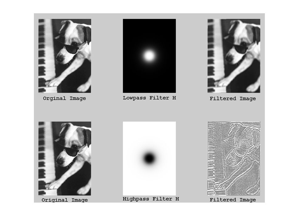
33. Frequency Domain Filters
Ideal Low Pass Filter
where d(u,v) is the distance of (u,v) from the centre of the filter and d0 is a positive number (the radius of the white circle).
for smoothing and blurring
Ideal High Pass Filter
for extracting the details of an image

34. Other Ideal Filters
The ideal bandpass filter retains the frequencies inside a given band and eliminates all the other.
The ideal bandreject filter eliminates the frequencies inside a given band and retains all the other.

35. Frequency Domain Filtering
Multiply by a filter in the
frequency domain <=>
convolve with the fiter in
spatial domain.
Fourier
Amplitude

36. Examples of ILPF FT Ringing and Blurring
Ideal in frequency domain means non-ideal in spatial domain, vice versa.

37. Butterworth Lowpass Filter
Transfer function
Where D0 = cut off frequency, n = filter order.

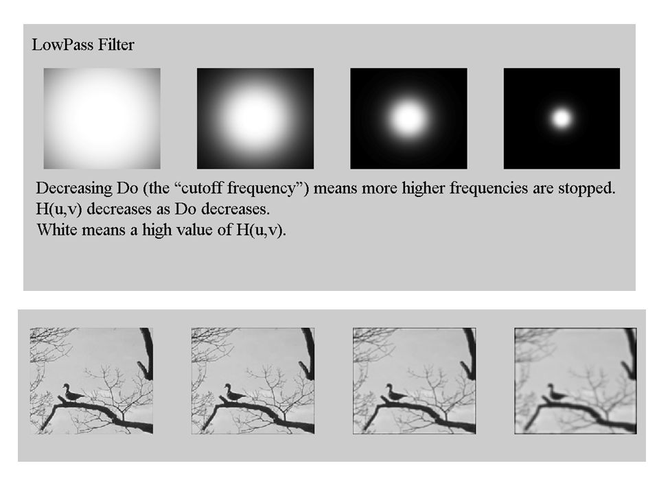
38. Notes on BLPF The image to be filtered is an MxN pixeled image
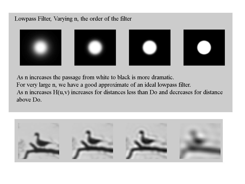
D(u,v) is the distance from the centre to the point (u,v), given by the formula
For a lowpass filter, this means that as D(u,v) increases, H(u,v) decreases. The effect is to dampen the higher frequencies which are represented as being a distance far from the centre and emphasise the lower frequencies which are represented by points close to the centre
D0 is known as the “cutoff” frequency. In an ideal lowpass filter, this is the point past which all frequencies would be eliminated.
Increasing D0 increases the number of frequencies that are “passed” (or lessens the dampening effects of higher frequencies)
Decreasing D0 means a smaller number of frequencies are allowed to pass (or the dampening effects of higher frequencies are increased). This would result in a more blurred image.
n is the order of the filter. Increasing n increases and decreases H(u,v) for D(u,v) less than and greater than D0 respectively, which means there is a dramatic passage from those frequencies which are kept and those which are dampened/eliminated. As n increases, H(u,v) nears zero when the value of D(u,v) is high. When n is very high, it is a good approximate of an ideal lowpass filter.

39. Results of BLPF There is less ringing effect compared to
those of ideal lowpass
filters!

40. Examples of IHPF
Ringing effect can be
obviously seen!

41. Butterworth High Pass Filters
The Butterworth high pass filter is given as:
where n is the order and D0 is the cut off distance as before 41

42. Results of BHPF

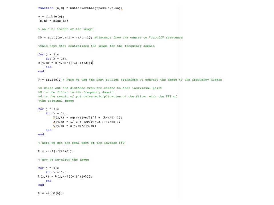
47. General Filtering Method
First we centre the image
Why?
What does that mean?
It means that when we apply the Fourier transform, the lowest frequencies will be in the centre and the highest frequencies will be around the edges.
Secondly we compute the Fourier Transform as above

48. General Filtering Method
Now we multiply by a filter function H(u,v), i.e.
(or if you’re fussy)
Note that this is not matrix multiplication. It is pointwise (or point by point) multiplication.
H(u,v) generally takes real values between 0 and 1
G(u,v) is complex-valued because F(u,v) is complex-valued

49. General Filtering Method
Calculate the Inverse Fourier Transform of G(u,v).
using the Inverse Fourier Transform formula
We then take the real part of g(x,y) (to remove any small complex residues)
This is then multiplied by (-1)x+y to realign the image again and produce the final filtered image.

50. Property of DFT - Separability
f(x,y)
Alternative 1
1-D DFT
by row
F(u,y)
1-D DFT
by column
Alternative 2
1-D DFT
by column
F(x,v)
F(u,v)
1-D DFT
by row

52. Enhancement vs. Restoration
A process which aims to improve bad images so they will “look” better
“Better” visual representation
Subjective
No quantitative measures
A process which aims to invert known or estimated degradation to images
Remove effects of sensing environment
Objective
Mathematical, model dependent quantitative measures

53. Inverse Filtering Simple (noiseless) case:
Then original image can be obtained by
Note: H(u,v) may have zero or near zero values in most parts of (u,v) range
at those points the division operation is undefined or results in meaningless values
for points having very small |H(u,v)|, although the division can be done, the noise will be amplified to an intolerable extent
restrict the area to low frequency part or use Gaussian weighting to solve this problem.

54. Acknowlegements
Slides are modified based on the original slide set from Dr Li Bai, The University of Nottingham, Jubilee Campus plus the following sources:
Digital Image Processing, by Gonzalez and Woods
Digital Image Processing, a practical introduction using Java by Nick Efford
An Intuitive Explanation of Fourier Theory