Download presentation
Presentation is loading. Please wait.

1
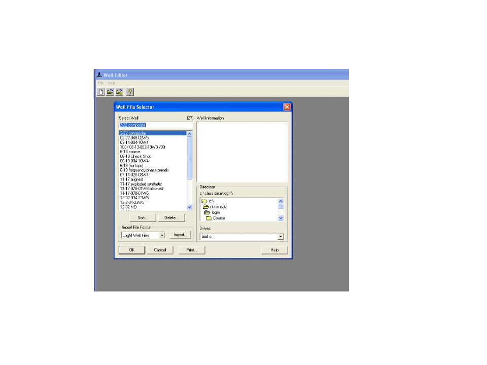
Course 4: Using AdvancedWell Editor Tools

2
Log curves are resampled

8
Best guess of what initial time shift should be Click apply to continue

9
Place and

10
The initial shift was a best guess that can be checked by undertaking a cross correlation

11
Select window of time

12
Improve correlation by shifting Use phase and time sliders

13
Window calculations to 0.95 to 1.56 and use phase and time sliders to maximize correlation coefficient OK

14
Ok to continue …

15
Zoom in on zone of interest and edit > time alignment

16
Click events in the synthetic and actual data to tie > Apply Once applied they are tied in, but you can click the undo button

17
File > Save As …

19
Checkshot obs at 100 to 200 m ints Travel paths include multiples, direct and reflections

20
Correct to true vertical depths

22
Tools > TVD editor

23
Select curves by draging mouse over them and apply > OK to return and File > Save as to save as LogM > OK

24
Name > OK > OK

25
Note TVD’s are a little less than MD File > Close All

26
Checkshot editor > Open well > Tools > Checkshot editor > add check shot times and depths to the table

27
File > save > Label (field data checkshots) > OK > Apply7
 > OK > Apply7")
28
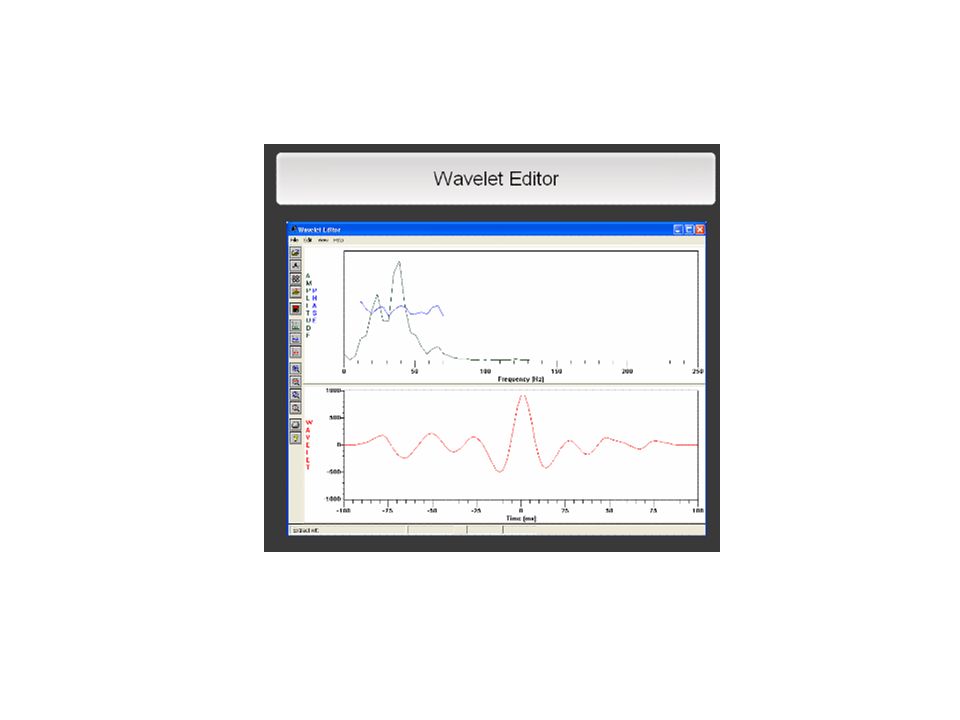
Note selections

29
View Vel from Corrected sonic then View > Fit Curve > have a look and exit

30
View > Select Curves > clear all> Select curves to display Sonic Cor sonic field Sonic Drift CS Vel Field Density Gr Adjust view

31
Note influence of TVD correction File > Save As

32
Align remaining wavelets Open File (original) Then View > Select Curves Clear All Sonic, Density and GR Switch to time mode (view time mode) Synthetics > synthetics > wavelets Place normal traces next to sonic log Activate check shot display corrected window
 Then View > Select Curves Clear All Sonic, Density and GR Switch to time mode (view time mode) Synthetics > synthetics > wavelets Place normal traces next to sonic log Activate check shot display corrected window")
33
Switch to time mode Create synthetic using corrected field check shots in the synthetic > Curve selection field. Wavelets Place your synthetic View > align wells option Use a formation top

34
Note differences in start time Then file > plot > default synthetic layout > select group 1

35
File > plot set up In schematic mode you can rearrange various boxes File > Exit Close all wells (file > close all) Exercise complete
 Exercise complete")
37
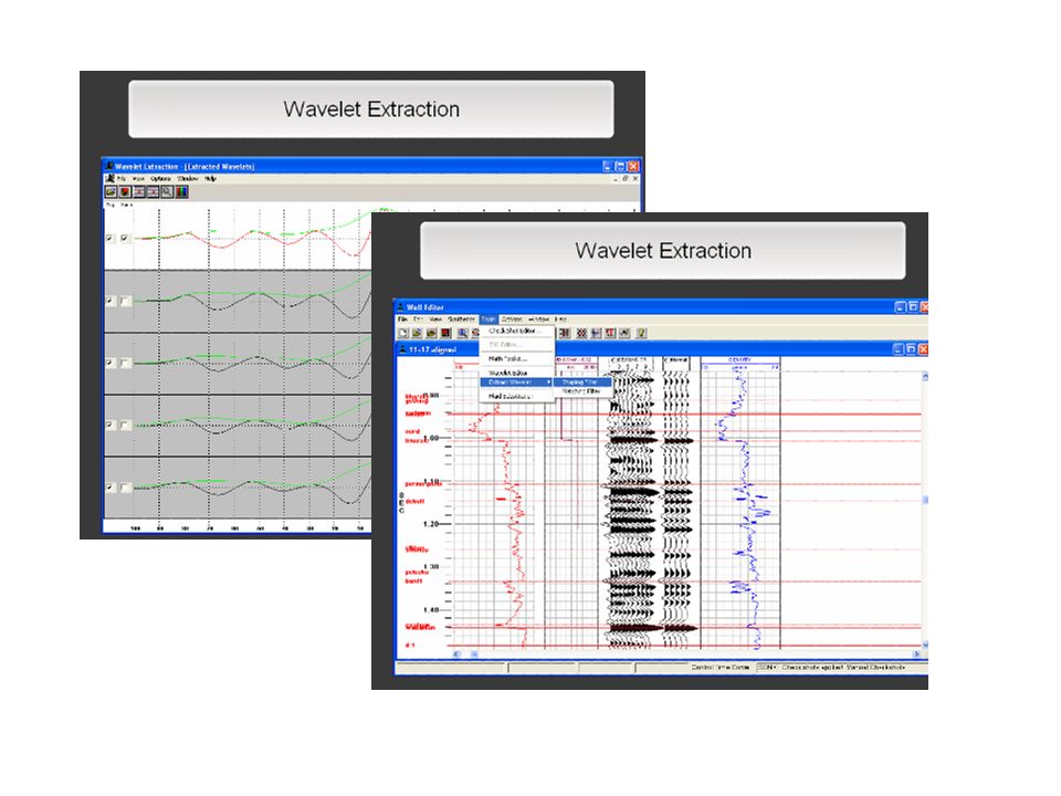
Open a well with synthetcs > Synthetics > Delete synthetic to delete synthetic panel if needed. For example to get rid of a synthetic usinga wavelet not considered realistic. Edit > Time depth controls Toggle on time/depth check box Change sample interval to 2 ms Apply shaping filter Tools > extract wavelet > shaping filter (uses reflection coefficients and seismic data)
.")
39
Now look at cross correltaion graph Align > cross correlation graph (from tool bar Align time and phase to maximize correlation. Now apply hsaping filter again Action > Set extraction data OK Action > Extract Wavelet > Weiner LEvenson

40
Focus on extracted wavelets

41
Options > align wavelets > automatic check box (on) > apply > close Options > Taper Bartlet Wavelet lengh 100, taper length 25 Options > Align Wavelets 3 for zero lag point > apply Click highlihgted area of display
 > apply > close Options > Taper Bartlet Wavelet lengh 100, taper length 25 Options > Align Wavelets 3 for zero lag point > apply Click highlihgted area of display")
42
Helps to center wavelets Close > File Save > Log M > Save average wavelet File > Exit

43
Synthetics > Synthetic Wavelets > File wavelet Open your wavelet file and > add Wavelet OK Locate normal traces on the display panel

44
Edit Wavelets Tools > Wavelet Editor > Select the extract file (wavelet you created Edit > Wavelet in the wavelet editor View > Show reference point Edit > Smooth

45
6 th icon from the top on the left hand toolbar Displays amplitude scale View > Scale (choose appropriate value OK to continue Edit > Draw

46
Draw in curve and click OK to continue redrawn

47
Phase > seventh icon down from the top Edit Smooth Define operator length (say 35) (note the methods available) Boc car used in this example> OK > note changes Save As > log M wavelet file type> give it a name > save > OK > exit To return to Well Editor screen
 (note the methods available) Boc car used in this example> OK > note changes Save As > log M wavelet file type> give it a name > save > OK > exit To return to Well Editor screen")
48
Create new synthetic using the corrected wavelet and compare Select Synthetics from Synthetic Wavelets> File Wavelet> browse to your new wavelet > select > Add Wavelet > OK Place synthetic (normal traces) > File close all
 > File close all")
49
Math tool kit will calculate a shale volume curve from the GR curve

50
Open file > In Well Editor Menu Bar select > Tools > Math Tool Kit Enter name, Create constant Click New > turn on imperial and metric values OK

51
Create another constant: New > All Shale 115 as metric and Imperial values Note existing curves and function box

52
Save and place the new curve From Edit > Log Scales select ShVol 0 to 100%, OK to apply and save

53
Generate a set of curves showing influence of water oil and gas in the formation First generate new shear sonic and Poisson ratio asuming 100% wet saturation

54
Create copy of your log display file (texas gas _ fluid sub > OK Now generate new curves Tools > fluid substitution Next (if accept the defaults)
")
55
Here we select the ShVol curve calculated in the previous exercise > next

56
Examine and finish Place the new curves Sh sonic in situ PR in situ Edit > Log Scales Shear sonic In Situ

57
Edit> Copy curve > to make copies of curves Density, sonic, sonic insitu, density and PR in situ Place Confirm name for new copy (numeral 1 appended) They will appear 1 x 1
 They will appear 1 x 1")
58
Next exercise we will recalculate Resize > tools > open Fluid substitution Turn off in-situ saturation 100% wet under VP/VS trends Enter start and end depths (ZOI) Next
 Next")
59
Under in-situ fluit properties select gas Enter brine salinity of 40,000 (ppm) Gas specific gravity 0.6 Constants > degrees centigrade Check pressure and change to 40,000 kPa Next
 Gas specific gravity 0.6 Constants > degrees centigrade Check pressure and change to 40,000 kPa Next")
60
View and Next Turn on the following check boxes and Finish

61
Click to place new porosity curve

62
EWdit curve header menu option to change labels They changed the copied 1’s to Wet others to gas Drag and drop curves on top of each other for comparison

63
Now – Oil substituted for gas Use the gas curves as input Edit > copy curve and make copies of all gas curves Select Density Gas PRInSitu Gas SHSonicInsitu Gas and Sonic Gas Then place (insert to left). You will get a series of proposed curve labels which you can change or OK Tools > Fluid Substitution Process > fluid substitution Enter start and end depths

64
Select Porosity and > LC Next Retains settings Select Pressure tab

65
Select substitute fluid properties tab & light oil Brine salinity to 40,000, 40 for oil gravity, change water saturation to 30% > Next

66
Make sure shale volume curve is selected Select desired output types finish

67
Edit curve header option to remane the 4 gas curves to oil curves > Close Drag and drop to compare water to gas to oil Save and give new ID … gas fluid sub final

68
End course 4

Similar presentations