1. Chapter 3 Introduction to Linear Programming

2. 3.1 What Is a Linear Programming Problem?
「線性」(linear),指模式中之所有函數均為線性函數；「規劃」(programming),指planning,而非 computer programming 中程式之意。
數學規劃(mathematical programming)是將問題以目標函數(object function)及限制式(constraint)等數學式表示出來的一種模式。當所有數學式均為線性時,則數學規劃即是線性規劃。
Linear Programming (LP,線性規劃) is a tool for solving optimization problems(最佳化問題).
Linear programming problems involve important terms that are used to describe linear programming.

3. Example 1: Giapetto’s Woodcarving
Giapetto manufactures wooden soldiers and trains.
Each soldier built:
Sell for $27 and uses $10 worth of raw materials.
Increase Giapetto’s variable labor/overhead costs by $14.
Requires 2 hours of finishing labor.
Requires 1 hour of carpentry labor.
Each train built:
Sell for $21 and used $9 worth of raw materials.
Increase Giapetto’s variable labor/overhead costs by $10.
Requires 1 hour of finishing labor.

4. Each week Giapetto can obtain:
All needed raw material.
Only 100 finishing hours.
Only 80 carpentry hours.
Demand for the trains is unlimited.
At most 40 soldiers are bought each week.
Giapetto wants to maximize weekly profit (revenues – costs).
Formulate a mathematical model of Giapetto’s situation that can be used maximize weekly profit.

5. Example 1: Solution
The Giapetto solution model incorporates the characteristics shared by all LP problems.
Decision variables(決策變數) should describe the decisions to be made.
x1 = number of soldiers produced each week
x2 = number of trains produced each week
The decision maker wants to maximize (usually revenue or profit) or minimize (usually costs) some function of the decision variables. This function to maximized or minimized is called the objective function(目標函數).
For the Giapetto problem, fixed costs do not depend upon the the values of x1 or x2.

6. Giapetto’s weekly profit can be expressed in terms of the decision variables x1 and x2:
Weekly profit =weekly revenue – weekly raw material costs – the weekly variable costs
= 3x1 + 2x2
Thus, Giapetto’s objective is to chose x1 and x2 to maximize weekly profit. The variable z denotes the objective function value of any LP.
Giapetto’s objective function is Maximize z = 3x1 + 2x2
The coefficient of an objective function variable is called an objective function coefficient (目標函數係數).

7. As x1 and x2 increase, Giapetto’s objective function grows larger.
For Giapetto, the values of x1 and x2 are limited by the following three restrictions called constraints(限制式) :
Each week, no more than 100 hours of finishing time may be used. (2 x1 + x2 ≤ 100)
Each week, no more than 80 hours of carpentry time may be used. (x1 + x2 ≤ 80)
Because of limited demand, at most 40 soldiers should be produced. (x1 ≤ 40)

8. The coefficients of the decision variables in the constraints are called the technological coefficient.
The number on the right-hand side of each constraint is called the constraint’s right-hand side (rhs, RHS，右手邊常數).
To formulate of an LP , the following question must be answered for each decision variable.
Can the decision variable only assume nonnegative (非負值) values, or is the decision variable allowed to assume both positive (正值), and negative (負值)values,?
If the decision variable can assume only nonnegative values, the sign restriction xi ≥ 0 is added.
If the variable can assume both positive and negative values, the decision variable xi is unrestricted in sign (urs，不受正負限制) .

9. For the Giapetto problem model, combining the sign restrictions x1≥0 and x2≥0 with the objective function and constraints yields the following optimization model:
Max z = 3x1 + 2x2 (objective function)
Subject to (s.t.)
2 x1 + x2 ≤ 100 (finishing constraint)
x1 + x2 ≤ 80 (carpentry constraint)
x ≤ 40 (constraint on demand for soldiers)
x ≥ (sign restriction)
x2 ≥ 0 (sign restriction)

10. Linear function & Linear inequalities
p.52
Linear function & Linear inequalities
A function f(x1, x2, …, xn of x1, x2, …, xn is a linear function(線性函數) if and only if for some set of constants, c1, c2, …, cn, f(x1, x2, …, xn) = c1x1 + c2x2 + … + cnxn.
For any linear function f(x1, x2, …, xn) and any number b, the inequalities f(x1, x2, …, xn) ≤ b and f(x1, x2, …, xn) ≥ b are linear inequalities (線性不等式).

11. p.53
Optimization
A LP problem is an optimization(最佳化) problem for which we do the following:
Attempt to maximize (or minimize) a linear function (called the objective function) of the decision variables.
The values of the decision variables must satisfy a set of constraints. Each constraint must be a linear equation or inequality.
A sign restriction is associated with each variable. For any variable xi, the sign restriction specifies either that xi must be nonnegative (xi ≥ 0) or that xi may be unrestricted in sign.

12. The objective function(目標函數) for an LP must be a linear function of the decision variables has two implications:
The contribution of the objective function from each decision variable is proportional(成比例性) to the value of the decision variable. For example, the contribution to the objective function for 4 soldiers is exactly fours times the contribution of 1 soldier.
The contribution to the objective function for any variable is independent(獨立) of the other decision variables. For example, no matter what the value of x2, the manufacture of x1 soldiers will always contribute 3x1 dollars to the objective function.

13. Each LP constraint(限制式) must be a linear inequality(線性不等式) or linear equation (線性等式) has two implications:
The contribution of each variable to the left-hand side of each constraint is proportional to the value of the variable. For example, it takes exactly 3 times as many finishing hours to manufacture 3 soldiers as it does 1 soldier.
The contribution of a variable to the left-hand side of each constraint is independent of the values of the variable. For example, no matter what the value of x1, the manufacture of x2 trains uses x2 finishing hours and x2 carpentry hours.

14. Linear Programming 之假設
Proportionality Assumption(成比例性假設) 指函數中,各個項目對於該函數之貢獻和變數之值成比例
Additivity Assumption (可加性假設) 指函數中,各個項目彼此獨立,因此相互可進行加減運算
Divisibility assumption (可分性假設) 要求所有變數可為任何實數,未必是整數
Certainty assumption (確定性假設) 所有係數均為已知常數 (objective function coefficients, right-hand side, and technological coefficients)

15. Proportionality Assumption (1)
目標函數中，產品獲得的利潤與產品的數量完全成固定比例
例如：生產1單位產品的利潤為100元， 生產2單位產品的利潤則為200元。
功能限制式中，生產產品所需的時間與數量完全成固定比例
例如：生產1單位需要3小時機器的時間， 生產2單位需要6小時機器的時間。

16. Proportionality Assumption (2)
對實務上問題，成比例性之假設未必成立。
當大量生產時，單位生產成本隨著生產數量之增加而降低(經濟規模) 。
學習曲線及設置成本等因素，使生產初期之單位生產成本高於生產後期之單位生產成本。
以市場考量，當稱產數量過多時，須降價銷售，單位利潤隨著生產數量之增加而遞減。
因此，應用線性規劃時，若違反太多成比例性之假設，則必須以其他方法，如：非線性規劃(nonlinear programming)，做為求解工具。(Chapter 11)

17. Additivity Assumption (1)
目標函數中，P1產品的利潤和P2產品的利潤彼此獨立，因此可相加而得到總利潤。
功能限制式中，無論生產多少P2產品，生產1單位P1產品均固定需要3小時機器的時間。

18. Additivity Assumption (2)
實際情況下，可加性有時也會有不適用的情形。
當產品相互競爭時，一產品銷售量增加，另一產品銷售量就會降低。
當產品有互補作用時，一產品銷售量增加，另一產品銷售量也提高。(例：電腦和印表機、粉筆和板擦)
製造過程中，也許兩產品的生產共同使用一台機器，此時若有規模經濟的現象，單位生產時間因生產數量增加而降低或機器需顯著的設置時間時，使得一產品的單位生產時間隨另一產品生產數量的增加而降低。若共同使用的機器有逐漸老舊現象，生產數量越多反而越慢，則一產品的單位生產時間隨著另一產品生產數量的增加而增加。
因此，應用線性規劃時，必須確認各函數中的各個項目是否完全獨立，確保可加性假設的合理性。

19. Divisibility Assumption
有些問題的變數必須是整數，例如，每天生產10部車。
在大多數情況下，當變數的值足夠大時，即使代表問題實際意義的變數必須是整數，只要將所得到的變數值取整數，以四捨五入、無條件捨去或無條件進入等方式，即可得到一個合理的整數解。 例如，若x1=10.6，則整數解x1=11 (四捨五入)。
當變數的值相當小時，或是當變數代表yes or no的意義時，則將所得到的實數取其整數，並不是可行的方法，此時以整數規劃（integer programming）求解。 (Chapter 9)

20. Certainty Assumption
係數不為隨機變數、機率值或不確定值。 例如,假設每生產1箱的產品可獲得$7,000利潤，此常數$7,000是假設為已知的。
在實際情況下，確定性假設經常無法完全滿足。
線性規劃大多數的係數都是對未來情況的預估值， 或多或少都會有不確定的成分。
大多數的係數隨著時間而不斷有小或大的變動。
求解線性規劃時，除了得到最佳解外，經常做敏感度分析（sensitivity analysis）以瞭解當係數變動時，最佳解會如何改變。(Chapter 5,6)

21. Feasible Region and Optimal Solution
The feasible region(可行區域) of an LP is the set of all points satisfying all the LP’s constraints and sign restrictions.
For a maximization problem, an optimal solution(最佳解) to an LP is a point in the feasible region with the largest objective function value.
Similarly, for a minimization problem, an optimal solution is a point in the feasible region with the smallest objective function value.

22. Exercise ： P.55 #1
Farmer Jones must determine how many acres of corn and wheat to plane this year. An acre of wheat yields 25 bushels of wheat and requires 10 hours of labor per week. An acre of corn yields 10 bushels of corn and requires 4 hours of labor per week. All wheat can be sold at 4$ a bushel, and all corn can be sold at $3 a bushel. Seven acres of land and 40 hours per week of labor are available. Government regulation require that at least 30 bushels of corn be produced during the current year. Let x1 = number of acres of corn planted, and x2 = number of acres of wheat planted. Using these decision variables, formulate an LP whose solution will tell Farmer Jones how to maximize the total revenue from wheat and corn.

23. Exercise ： P.55 #1
x1 = number of acres of corn planted x2 = number of acres of wheat planted
max z = 30x x2
s.t. x x2  (Land Constraint)
4x1 + 10x2  (Labor Constraint)
10x  (Govt. Constraint)
x1  0, x2  0

24. Exercise ： P.55 #3
x1= number of bushels of corn produced 1 bushel of corn uses 1/10 acre of land and 4/10 hours of labor
x2= number of bushels of wheat produced 1 bushel of wheat uses 1/25 acre of land and 10/25 hours of labor
max z = 3x1 + 4x2
s.t x1/10 + x2/  (Land Constraint)
4x1/ x2/25  (Labor Const.)
x  (Govt. Const.)
x1  0, x2  0

25. Exercise ： P.55 #4
Truckco manufactures two types of trucks: 1 and 2. Each truck must go through the painting shop and assembly shop. If the painting shop were completely devoted to painting Type 1 trucks, then 800 per day could be painted; if the painting shop were completely devoted to painting Type 2 trucks, then 700 per day could be painted.
If the assembly shop were completely devoted to assembling truck 1 engines, then 1,500 per day could be assembled; if the assembly shop were completely devoted to assembling truck 2 engines, then 1,200 per day could be assembled.
Each Type 1 truck contributes $300 to profit;
Each Type 2 truck contributes $500,
Formulate an LP that will maximize Truckco’s profit.

26. Exercise：p.55 #5
Why don’t we allow an LP to have < or > constraints?

27. To Find solution by the followings：
Graphical method (圖解法)
若LP只有兩個變數，則以下列三步驟求解：
STEP 1. 繪製非負限制式(或不受正負限制)之範圍
STEP 2. 繪製各功能限制式之範圍，並決定可行區域
STEP 3. 繪製目標函數之線條，並決定最佳解
Algebra method (代數法)
Simplex method (單體法) (Chapter 4)

28. 3.2 The Graphical Solution to a Two-Variable LP Problem
Any LP with only two variables can be solved graphically (圖解).
The variables are always labeled x1 and x2 and the coordinate axes the x1 and x2 axes.
Satisfies 2x1 + 3x2 ≥ 6
Satisfies 2x1 + 3x2 ≤ 6
P.56 Fig. 1

29. Since the Giapetto LP has two variables, it may be solved graphically.
The feasible region is the set of all points satisfying the constraints.
2 x1 + x2 ≤ (finishing constraint)
x1 + x2 ≤ (carpentry constraint)
x1 ≤ (demand constraint)
x1 ≥ (sign restriction)
x2 ≥ (sign restriction)

30. The set of points satisfying the Giapetto LP is bounded by the five sided polygon DGFEH. Any point on or in the interior of this polygon (the shade area) is in the feasible region.
P.57 Fig. 2

31. Having identified the feasible region for the Giapetto LP, a search can begin for the optimal solution which will be the point in the feasible region with the largest z-value.
To find the optimal solution, graph a line on which the points have the same z-value. In a max problem, such a line is called an isoprofit line while in a min problem, this is called the isocost line. The figure shows the isoprofit lines for z = 60, z = 100, and z = 180

32. A constraint is binding if the left-hand and right-hand side of the constraint are equal when the optimal values of the decision variables are substituted into the constraint.
In the Giapetto LP, the finishing and carpentry constraints are binding.
A constraint is nonbinding if the left-hand side and the right-hand side of the constraint are unequal when the optimal values of the decision variables are substituted into the constraint.
In the Giapetto LP, the demand constraint for wooden soldiers is nonbinding since at the optimal solution (x1 = 20), x1 < 40.

33. 線性函數之性質
P.59 Fig. 3

34. Exercise : which are convex sets？
（○）
（○）
（×）
（×）

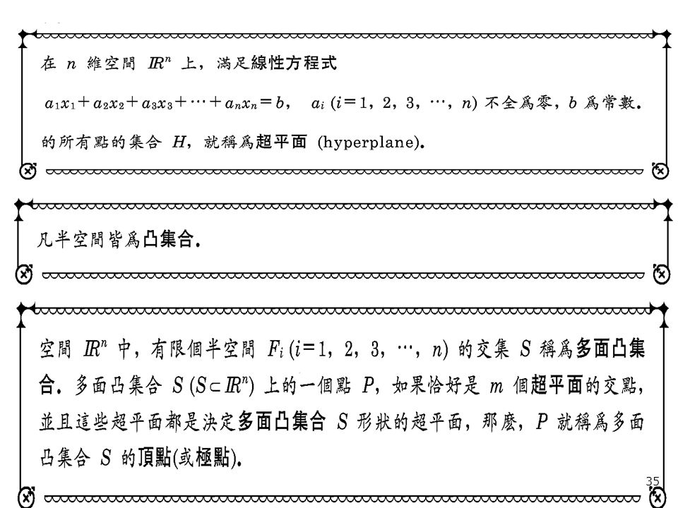
37. p.59
A set of points S is a convex (凸集合) set if the line segment jointing any two pairs of points in S is wholly contained in S.
For any convex set S, a point p in S is an extreme point (極點) if each line segment that lines completely in S and contains the point P has P as an endpoint of the line segment.
Extreme points are sometimes called corner points (角點),, because if the set S is a polygon, the extreme points will be the vertices, or corners, of the polygon.
The feasible region for the Giapetto LP will be a convex set.

38. p.60
Example 2 : Dorian Auto
Dorian Auto manufactures luxury cars and trucks.
The company believes that its most likely customers are high-income women and men.
To reach these groups, Dorian Auto has embarked on an ambitious TV advertising campaign and will purchase 1-mimute commercial spots on two type of programs: comedy shows and football games.

39. Each comedy commercial is seen by 7 million high income women and 2 million high-income men and costs $50,000.
Each football game is seen by 2 million high-income women and 12 million high-income men and costs $100,000.
Dorian Auto would like for commercials to be seen by at least 28 million high-income women and 24 million high-income men.
Use LP to determine how Dorian Auto can meet its advertising requirements at minimum cost.

40. Example 2: Solution
Dorian decides how many comedy and football ads should be purchased, so the decision variables are
x1 = number of 1-minute comedy ads
x2 = number of 1-minute football ads
Dorian wants to minimize total advertising cost.
The objective functions is min z = 50 x x2
Dorian faces the following the constraints.
Commercials must reach at least 28 million high-income women. (7x1 + 2x2 ≥ 28)
Commercials must reach at least 24 million high-income men. (2x1 + 12x2 ≥ 24)
The sign restrictions are necessary, so x1, x2 ≥ 0.

41. Like the Giapetto LP, The Dorian LP has a convex feasible region (p
Like the Giapetto LP, The Dorian LP has a convex feasible region (p.61 Fig.4).
The feasible region for the Dorian problem, however, contains points for which the value of at least one variable can assume arbitrarily large values.
Such a feasible region is called an unbounded feasible region (無窮可行區域).

42. To solve this LP graphically begin by graphing the feasible region.
min z = 50 x x2
s.t. 7x1 + 2x2 ≥ 28
2x1 + 12x2 ≥ 24
x1, x2 ≥ 0.
p.61 Figure 4

43. Since Dorian wants to minimize total advertising costs, the optimal solution to the problem is the point in the feasible region with the smallest z value.
An isocost line with the smallest z value passes through point E and is the optimal solution at x1 = 3.6 and x2 = 1.4.
Both the high-income women and high-income men constraints are satisfied, both constraints are binding.

44. Does the Dorian model meet the four assumptions of LP?
The Proportionality Assumption is violated because at a certain point advertising yields diminishing returns.
Even though the Additivity Assumption was used in writing: (Total viewers) = (Comedy viewer ads) + (Football ad viewers) many of the same people might view both ads, double-counting of such people would occur thereby violating the assumption.
The Divisibility Assumption is violated if only 1-minute commercials are available. Dorian is unable to purchase 3.6 comedy and 1.4 football commercials.
The Certainty assumption is also violated because there is no way to know with certainty how many viewers are added by each type of commercial.

45. Exercise：p.63 #1~#6 Graphically solved problem 1 of page 55.
(Exercise of slice 22)

46. p.63
3.3 Special Cases
The Giapetto and Dorian LPs each had a unique optimal solution.
Some types of LPs do not have unique solutions.
Some LPs have an infinite number of solutions (alternative optimal solutions ,擇一最佳解 or multiple optimal solutions ,多重最佳解).
Some LPs have no feasible solutions (infeasible solutions,無解).
Some LP are unbounded.There are points in the feasible region with arbitrarily large (in a max problem) z-values. (unbounded solution,無窮解)

47. The technique of goal programming is often used to choose among alternative optimal solutions.
no feasible solutions and unbounded solution are called no optimal solutions(無最佳解).
It is possible for an LP’s feasible region to be empty, resulting in an infeasible LP.
Because the optimal solution to an LP is the best point in the feasible region, an infeasible LP has no optimal solution.
For a max problem, an unbounded LP occurs if it is possible to find points in the feasible region with arbitrarily large z-values, which corresponds to a decision maker earning arbitrarily large revenues or profits.

48. Other Examples：
Alternative Optimal Solutions Example 3 (p.63 Fig.5)

49. Other Examples：
Infeasible Solution Example 4 (p.65, Fig.6)

50. Other Examples：
Unbounded Solution Example 5 (p.67, Fig.7)

51. p.67
Every LP with 2-variables must fall into one of the following four cases.
The LP has a unique optimal solution.
The LP has alternative or multiple optimal solutions: Two or more extreme points are optimal, and the LP will have an infinite number of optimal solutions.
The LP is infeasible: The feasible region contains no points.
The LP unbounded: There are points in the feasible region with arbitrarily large z-values (max problem) or arbitrarily small z-values (min problem).

52. Exercise 1：p.68 #1 Graphically solve the following LP：
No feasible solution

53. Exercise 2： p.68 #2 Graphically solve the following LP：
Alternative optimal solutions

54. Exercise 3： p.68 #3 Graphically solve the following LP：
Unbounded solution

55. Exercise 4： p.68 #4 Graphically solve the following LP：
x1 = 3, x2 = 0, z = 9

56. Example 6: Diet Problem (飲食問題)
以最低成本滿足各種營養成分的要求
一般農場之牛羊雞鴨飼養
My diet requires that all the food I get come from one of the four “basic food groups”.
The following four foods are available for consumption: brownies, chocolate ice cream, cola and pineapple cheesecake.
Each brownie costs 50¢, each scoop of chocolate ice cream costs 20¢, each bottle of cola costs 30¢, and each piece of pineapple cheesecake costs 80¢.
Each day, I must ingest at least 500 calories, 6 oz of chocolate, 10 oz of sugar, and 8 oz of fat.

57. The nutritional content per unit of each food is given. (Table 2)
Formulate a linear programming model that can be used to satisfy my daily nutritional requirements at minimum cost.
Table 2
Type of food
Calories
Chocolate
Sugar
Fat
Brownie
400 3 2
Chocolate ice cream
200 4
Cola
150 1
Pineapple
500 5

58. Example 6: Solution We define the decision variables:
x1 = number of brownies eaten daily
x2 = number of scoops of chocolate ice cream eaten daily
x3 = bottles of cola drunk daily
x4 = pieces of pineapple cheesecake eaten daily

59. My objective is to minimize the cost of my diet.
The total cost of any diet may be determined from the following relation: (total cost of diet) = (cost of brownies) (cost of ice cream) (cost of cola) (cost of cheesecake).
The decision variables must satisfy four constraints:
Daily calorie intake must be at least 500 calories.
Daily chocolate intake must be at least 6 oz.
Daily sugar intake must be at least 10 oz.
Daily fat intake must be at least 8 oz.

60. Table 2 Type of food Calories Chocolate Sugar Fat Cost (¢) No. of food
Brownie
400 3 2 50 x1
Ice cream
200 4 20 x2
Cola
100 1 30 x3
Pineapple
cheesecake
500 5 80 x4
constraints
500 6
10 8

61. Example 6：
The optimal solution x1=x4=0, x2=3, x3=1, z=90

62. Exercise：p.71 #2
Table 3.
Let x1 = Number of valves ordered each month from supplier 1
x2 = Number of valves ordered each month from supplier 2
x3 = Number of valves ordered each month from supplier 3

63. Table 3
Supplier L M S
Cost
No. of valve 1 40 20 5 x1 2 30 35 4 x2 3 60 x3
constraint
 500
 300
xi  700
min z = 5x1 + 4x2 + 3x3
s.t x x x3  500
0.4x x x3  300
0.2x x x3  300
x1  700, x2  700, x3  700
x1  0, x2  0, x3  0

64. 3.5 A Work-Scheduling Problem (人力安排問題)
管理者如何在不同時段,安排適當之人力,以滿足人力需求,並使人事成本最低？
Many applications of linear programming involve determining the minimum-cost method for satisfying workforce requirements.
One type of work scheduling problem is a static scheduling problem.
In reality, demands change over time, workers take vacations in the summer, and so on, so the post office does not face the same situation each week. This is a dynamic scheduling problem.
Example 7. Table 4.

65. A post office requires different numbers of full-time employees on different days of the week. The number of full-time employees required on each day is given in Table 4. Union rules state that each full-time employee must work five consecutive days and then receive two days off. For example, an employee who works Monday to Friday must be off on Saturday and Sunday. The post office wants to meet its daily requirements using only full-time employees. Formulate an LP that the post office can use to minimize the number of full-time employees who must be hired.

66. Example 7：Post Office problem(1)
Let xi= number of employees beginning work on day i
Min z = x1+x2+x3+x4+x5+x6+x7
s.t. x x4+x5+x6+x7  17 (Monday constraint)
x1+x x5+x6+x7  13 (Tuesday constraint)
x1+x2+x x6+x7  15 (Wednesday constraint)
x1+x2+x3+x x7  19 (Thursday constraint)
x1+x2+x3+x4+x  14 (Friday constraint)
x2+x3+x4+x5+x  16 (Saturday constraint)
x3+x4+x5+x6+x7  11 (Sunday constraint)
xi  0 ( i = 1,2,3,4,5,6,7) (sign restrictions)

67. The optimal solution is
To find a reasonable answer in which all variables are integers.

68. Exercise：p.75
Let x1 = Number of fulltime employees (FTE) who start work on Sunday x2 = Number of FTE who start work on Monday
： x7 = Number of FTE who start work on Saturday x8 = Number of part‑time employees (PTE) who start work on Sunday ： x14 = Number of PTE who start work on Saturday

69. min z = 15(8)(5)(x1 + x2 + ...x7)+10(4)(5)(x8 + ...x14)
s.t. 8(x1+x4+x5+x6+x7)+4(x8+x11+x12+x13+x14)  88 (Sunday)
8(x1+x2+x5+x6+x7)+4(x8+x9+x12+x13+x14)  136 (Monday)
8(x1+x2+x3+x6+x7)+4(x8+x9+x10+x13+x14)  104 (Tuesday)
8(x1+x2+x3+x4+x7)+4(x8+x9+x10+x11+x14)  120 (Wednesday)
8(x1+x2+x3+x4+x5)+4(x8+x9+x10+x11+x12)  152 (Thursday)
8(x2+x3+x4+x5+x6)+4(x9+x10+x11+x12+x13)  112 (Friday)
8(x3+x4+x5+x6+x7)+4(x10+x11+x12+x13+x14)  128 (Saturday)
20(x8+x9+x10+x11+x12+x13+x14)  ( )
All variables 0.
(this constraint ensures that part‑time labor will fulfill at most 25% of all labor requirements)

70. 3.8 Blending Problems(混合問題)
將不同原料以一定比例混合,產生所要求之產品
Situations in which various inputs must be blended in desired proportion to produce goods for sale are often amenable to linear programming analysis.
Some examples of how linear programming has been used to solve blending problems.
Blending various types of crude oils to produce different types of gasoline and other outputs.
Blending various chemicals to produce other chemicals
Blending various types of metal alloys to produce various types of steels

71. Example 12：Oil Blending p.86 Table 12 Table 13 Gas
Sales Price per Barrel($)
Crude
Purchase Price per Barrel ($) 1 70 45 2 60 35 3 50 25
Table 13
Crude
Octane
rating
Sulfur
Content(%) 1 12
0.5 2 6
2.0 3 8
3.0

72. Exercise：problem 1 of page 92
Let Ing. 1 = Sugar, Ing. 2 = Nuts, Ing. 3 = Chocolate, Candy 1 = Slugger and Candy 2 = Easy Out.
Let xij = Ounces of Ing. i used to make candy j.
max z = 25(x12 + x22 + x32) + 20(x11 + x21 + x31)
s.t. x11 + x12  100 (Sugar Const.)
x21 + x22  20 (Nuts Constraint)
x31 + x32  30 (Chocolate Const.)
x22/(x12 + x22 + x32)  
x21/(x11 + x21 + x31)  
x31/(x11 + x21 + x31)  
 are not LP constraints and should be replaced .
Replace  by x220.2(x12+x22+x32) or 0.8x22‑0.2x12‑0.2x32  0
Replace  by x210.1(x11+x21+x31) or 0.9x21‑0.1x11‑0.1x31  0
Replace  by x310.1(x11+x21+x31) or 0.9x31‑0.1x11‑0.1x21  0