1. CCMIII U2D4 Warmup This graph of a linear programming model consists of polygon ABCD and its interior. Under these constraints, at which point does the minimum value of 3x + 2y occur? A. A B. B C. C D. D

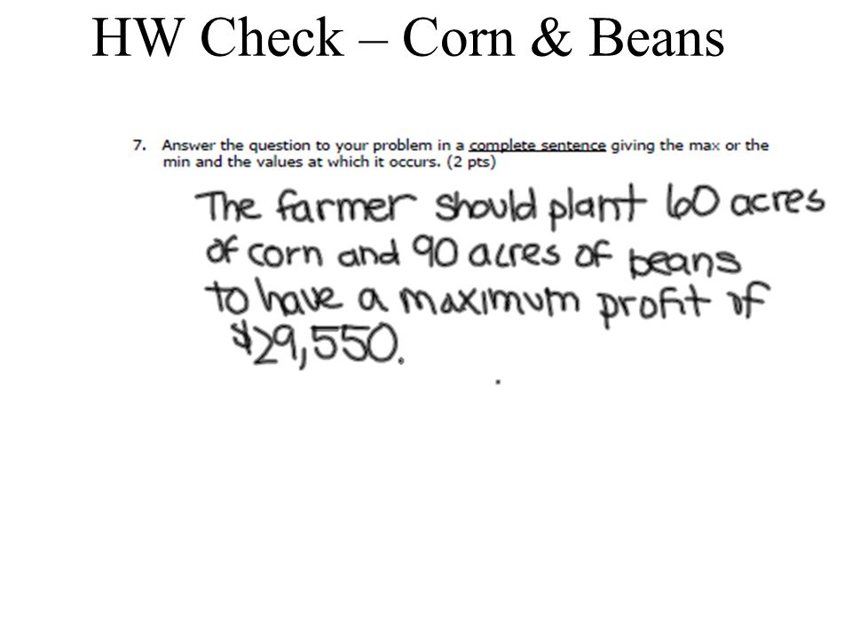
2. HW Check – Corn & Beans

7. 7 Continue Introduction to Linear Programming

8. M3U2D4 Linear Programming Cont. OBJECTIVES: Determine feasible regions pertaining to maximum and minimum conditions Use geometric methods to solve multi – step problems

10. Decision Variables Represent the quantities that a manager can change

11. Objective Function The equation that represents the goal of either maximizing profit or minimizing cost

12. Constraints Limitations created by scarce resources (time, equipment, etc.) Expressed algebraically by inequalities

13. Feasible Region Area containing all the points that satisfy the constraints All possible solutions to the problem lie in the feasible region or on the boundary.

14. Corner Points The optimal solution will always lie on a corner of the feasible region.

15. 15 Shoes Activity Complete in pairs by playing cards

16. 16 Shoes Activity Key

17. 17 Shoes Activity Key

18. 18 Shoes Activity Key

19. 19 Shoes Activity Key

20. Homework Linear Programming Reteaching WS front and back Additional slides on Linear Programming follow. Students- you should refer to these if you need further clarification.

21. 21 Example of Linear Programming Problem Each week the company can obtain: All needed raw material. Only 100 finishing hours. Only 80 carpentry hours. Also: Demand for the trains is unlimited. At most 40 soldiers are bought each week. Giapetto wants to maximize weekly profit (revenues – expenses). Formulate a mathematical model of Giapetto’s situation that can be used maximize weekly profit.

22. 22 Example of Linear Programming Problem The Giapetto solution model incorporates the characteristics shared by all linear programming problems. Decision Variables x 1 = # of soldiers produced each week x 2 = # of trains produced each week Objective Function The decision maker wants to maximize (usually revenue or profit) or minimize (usually costs) some function of the decision variables.

23. 23 Example of Linear Programming Problem Company’s weekly profit can be expressed in terms of the decision variables x 1 and x 2 : Weekly profit = weekly revenue – weekly raw material costs – the weekly variable costs Weekly profit = (27x 1 + 21x 2 ) – (10x 1 + 9x 2 ) – (14x 1 + 10x 2 ) = 3x 1 + 2x 2

24. 24 Example of Linear Programming Problem Constraint 1 Each week, no more than 100 hours of finishing time may be used. 2 x 1 + x 2 ≤ 100 Constraint 2 Each week, no more than 80 hours of carpentry time may be used. x 1 + x 2 ≤ 80 Constraint 3 Because of limited demand, at most 40 soldiers should be produced. x 1 ≤ 40

25. 25 Example of Linear Programming Problem Sign Restrictions If the decision variable can assume only nonnegative values, the sign restriction x i ≥ 0 is added. If the variable can assume both positive and negative values, the decision variable x i is unrestricted in sign (often abbreviated urs). The coefficients of the constraints are often called the technological coefficients. The number on the right-hand side of the constraint is called the constraint’s right-hand side (or rhs).

26. 26 Example of Linear Programming Problem optimization model: Max z = 3x 1 + 2x 2 (objective function) Subject to (s.t.) 2 x 1 + x 2 ≤ 100(finishing constraint) x 1 + x 2 ≤ 80(carpentry constraint) x 1 ≤ 40(constraint on demand for soldiers) x 1 ≥ 0(sign restriction) x 2 ≥ 0(sign restriction)

27. 27 What Is a Linear Programming Problem? 1. Attempt to maximize (or minimize) a linear function (called the objective function) of the decision variables. 2. The values of the decision variables must satisfy a set of constraints. 3. Each constraint must be a linear equation or inequality. 4. A sign restriction is associated with each variable. For each variable x i, the sign restriction specifies either that x i must be nonnegative (x i ≥ 0) or that x i may be unrestricted in sign. A linear programming problem (LP) is an optimization problem for which we do the following:

28. 28 Assumptions of Linear Programming Proportionality and Additive Assumptions The objective function for an LP must be a linear function of the decision variables has two implications: 1. The contribution of the objective function from each decision variable is proportional to the value of the decision variable. 2. The contribution to the objective function for any variable is independent of the other decision variables.

29. 29 Assumptions of Linear Programming 1. The contribution of each variable to the left-hand side of each constraint is proportional to the value of the variable. 2. The contribution of a variable to the left-hand side of each constraint is independent of the values of the variable. Each LP constraint must be a linear inequality or linear equation has two implications:

30. 30 Assumptions of Linear Programming Divisibility Assumption The divisibility assumption requires that each decision variable be permitted to assume fractional values. The Certainty Assumption The certainty assumption is that each parameter (objective function coefficients, right-hand side, and technological coefficients) are known with certainty.

31. 31 2.1 - What Is a Linear Programming Problem? Feasible Region and Optimal Solution Give a point in feasible region Give a point that is not in feasible region Giapetto Constraints 2 x 1 + x 2 ≤ 100 (finishing constraint) x 1 + x 2 ≤ 80 (carpentry constraint) x 1 ≤ 40 (demand constraint) x 1 ≥ 0 (sign restriction) x 2 ≥ 0 (sign restriction) The feasible region of an LP is the set of all points satisfying all the LP’s constraints and sign restrictions.

32. 32 What Is a Linear Programming Problem? For a maximization problem, an optimal solution to an LP is a point in the feasible region with the largest objective function value. Similarly, for a minimization problem, an optimal solution is a point in the feasible region with the smallest objective function value. Most LPs have only one optimal solution. However, some LPs have no optimal solution, and some LPs have an infinite number of solutions.

33. 33 2.2 – Graphical Solution to a 2-Variable LP Finding the Feasible Solution Since the Giapetto LP has two variables, it may be solved graphically. The feasible region is the set of all points satisfying the constraints: Giapetto Constraints 2 x 1 + x 2 ≤ 100 (finishing constraint) x 1 + x 2 ≤ 80 (carpentry constraint) x 1 ≤ 40 (demand constraint) x 1 ≥ 0 (sign restriction) x 2 ≥ 0 (sign restriction) A graph of the constraints and feasible region is shown on the next slide.

34. 34 Graphical Solution to a 2-Variable LP Any point on or in the interior of the five sided polygon DGFEH(the shade area) is in the feasible region. Isoprofit line for maximization problem (Isocost line for minimization problem )is a set of points that have the same z-value

35. 35 Two type of Constraints Binding and Nonbinding constraints A constraint is binding if the left-hand and right- hand side of the constraint are equal when the optimal values of the decision variables are substituted into the constraint.

36. 36 Two type of Constraints A constraint is nonbinding if the left- hand side and the right-hand side of the constraint are unequal when the optimal values of the decision variables are substituted into the constraint.

37. 37 Special Cases of Graphical Solution Some LPs have an infinite number of solutions (alternative or multiple optimal solutions). Some LPs have no feasible solution (infeasible LPs). Some LPs are unbounded: There are points in the feasible region with arbitrarily large (in a maximization problem) z-values.

38. 38 Alternative or Multiple Solutions Any point (solution) falling on line segment AE will yield an optimal solution with the same objective value

39. 39 no feasible solution No feasible region exists Some LPs have no solution. Consider the following formulation:

40. 40 Unbounded LP The constraints are satisfied by all points bounded by the x 2 axis and on or above AB and CD. There are points in the feasible region which will produce arbitrarily large z-values (unbounded LP).