Download presentation
Presentation is loading. Please wait.

1
SPSS Instructions for Introduction to Biostatistics Larry Winner Department of Statistics University of Florida

2
SPSS Windows Data View –Used to display data –Columns represent variables –Rows represent individual units or groups of units that share common values of variables Variable View –Used to display information on variables in dataset –TYPE: Allows for various styles of displaying –LABEL: Allows for longer description of variable name –VALUES: Allows for longer description of variable levels –MEASURE: Allows choice of measurement scale Output View –Displays Results of analyses/graphs

3
Data Entry Tips I For variables that are not identifiers (such as name, county, school, etc), use numeric values for levels and use the VALUES option in VARIABLE VIEW to give their levels. Some procedures require numeric labels for levels. SPSS will print the VALUES on output For large datasets, use a spreadsheet such as EXCEL which is more flexible for data entry, and import the file into SPSS Give descriptive LABEL to variable names in the VARIABLE VIEW Keep in mind that Columns are Variables, you don’t want multiple columns with the same variable

4
Data Entry/Analysis Tips II When re-analyzing previously published data, it is often possible to have only a few outcomes (especially with categorical data), with many individuals sharing the same outcomes (as in contingency tables) For ease of data entry: –Create one line for each combination of factor levels –Create a new variable representing a COUNT of the number of individuals sharing this “outcome” When analyzing data Click on: –DATA WEIGHT CASES WEIGHT CASES BY –Click on the variable representing COUNT –All subsequent analyses treat that outcome as if it occurred COUNT times
, with many individuals sharing the same outcomes (as in contingency tables) For ease of data entry: –Create one line for each combination of factor levels –Create a new variable representing a COUNT of the number of individuals sharing this outcome When analyzing data Click on: –DATA WEIGHT CASES WEIGHT CASES BY –Click on the variable representing COUNT –All subsequent analyses treat that outcome as if it occurred COUNT times")
5
Example 1.3 - Grapefruit Juice Study To import an EXCEL file, click on: FILE OPEN DATA then change FILES OF TYPE to EXCEL (.xls) To import a TEXT or DATA file, click on: FILE OPEN DATA then change FILES OF TYPE to TEXT (.txt) or DATA (.dat) You will be prompted through a series of dialog boxes to import dataset
 To import a TEXT or DATA file, click on: FILE OPEN DATA then change FILES OF TYPE to TEXT (.txt) or DATA (.dat) You will be prompted through a series of dialog boxes to import dataset")
6
Descriptive Statistics-Numeric Data After Importing your dataset, and providing names to variables, click on: ANALYZE DESCRIPTIVE STATISTICS DESCRIPTIVES Choose any variables to be analyzed and place them in box on right Options include:

7
Example 1.3 - Grapefruit Juice Study

8
Descriptive Statistics-General Data After Importing your dataset, and providing names to variables, click on: ANALYZE DESCRIPTIVE STATISTICS FREQUENCIES Choose any variables to be analyzed and place them in box on right Options include (For Categorical Variables): –Frequency Tables –Pie Charts, Bar Charts Options include (For Numeric Variables) –Frequency Tables (Useful for discrete data) –Measures of Central Tendency, Dispersion, Percentiles –Pie Charts, Histograms
: –Frequency Tables –Pie Charts, Bar Charts Options include (For Numeric Variables) –Frequency Tables (Useful for discrete data) –Measures of Central Tendency, Dispersion, Percentiles –Pie Charts, Histograms")
9
Example 1.4 - Smoking Status

10
Vertical Bar Charts and Pie Charts After Importing your dataset, and providing names to variables, click on: GRAPHS BAR… SIMPLE (Summaries for Groups of Cases) DEFINE Bars Represent N of Cases (or % of Cases) Put the variable of interest as the CATEGORY AXIS GRAPHS PIE… (Summaries for Groups of Cases) DEFINE Slices Represent N of Cases (or % of Cases) Put the variable of interest as the DEFINE SLICES BY
 DEFINE Bars Represent N of Cases (or % of Cases) Put the variable of interest as the CATEGORY AXIS GRAPHS PIE… (Summaries for Groups of Cases) DEFINE Slices Represent N of Cases (or % of Cases) Put the variable of interest as the DEFINE SLICES BY")
11
Example 1.5 - Antibiotic Study

12
Histograms After Importing your dataset, and providing names to variables, click on: GRAPHS HISTOGRAM Select Variable to be plotted Click on DISPLAY NORMAL CURVE if you want a normal curve superimposed (see Chapter 3).
.")
13
Example 1.6 - Drug Approval Times

14
Side-by-Side Bar Charts After Importing your dataset, and providing names to variables, click on: GRAPHS BAR… Clustered (Summaries for Groups of Cases) DEFINE Bars Represent N of Cases (or % of Cases) CATEGORY AXIS: Variable that represents groups to be compared (independent variable) DEFINE CLUSTERS BY: Variable that represents outcomes of interest (dependent variable)
 DEFINE Bars Represent N of Cases (or % of Cases) CATEGORY AXIS: Variable that represents groups to be compared (independent variable) DEFINE CLUSTERS BY: Variable that represents outcomes of interest (dependent variable)")
15
Example 1.7 - Streptomycin Study

16
Scatterplots After Importing your dataset, and providing names to variables, click on: GRAPHS SCATTER SIMPLE DEFINE For Y-AXIS, choose the Dependent (Response) Variable For X-AXIS, choose the Independent (Explanatory) Variable
 Variable For X-AXIS, choose the Independent (Explanatory) Variable")
17
Example 1.8 - Theophylline Clearance

18
Scatterplots with 2 Independent Variables After Importing your dataset, and providing names to variables, click on: GRAPHS SCATTER SIMPLE DEFINE For Y-AXIS, choose the Dependent Variable For X-AXIS, choose the Independent Variable with the most levels For SET MARKERS BY, choose the Independent Variable with the fewest levels

19
Example 1.8 - Theophylline Clearance

20
Contingency Tables for Conditional Probabilities After Importing your dataset, and providing names to variables, click on: ANALYZE DESCRIPTIVE STATISTICS CROSSTABS For ROWS, select the variable you are conditioning on (Independent Variable) For COLUMNS, select the variable you are finding the conditional probability of (Dependent Variable) Click on CELLS Click on ROW Percentages
 For COLUMNS, select the variable you are finding the conditional probability of (Dependent Variable) Click on CELLS Click on ROW Percentages")
21
Example 1.10 - Alcohol & Mortality

22
Independent Sample t-Test After Importing your dataset, and providing names to variables, click on: ANALYZE COMPARE MEANS INDEPENDENT SAMPLES T-TEST For TEST VARIABLE, Select the dependent (response) variable(s) For GROUPING VARIABLE, Select the independent variable. Then define the names of the 2 levels to be compared (this can be used even when the full dataset has more than 2 levels for independent variable).
..")
23
Example 3.5 - Levocabastine in Renal Patients

24
Wilcoxon Rank-Sum/Mann-Whitney Tests After Importing your dataset, and providing names to variables, click on: ANALYZE NONPARAMETRIC TESTS 2 INDEPENDENT SAMPLES For TEST VARIABLE, Select the dependent (response) variable(s) For GROUPING VARIABLE, Select the independent variable. Then define the names of the 2 levels to be compared (this can be used even when the full dataset has more than 2 levels for independent variable). Click on MANN-WHITNEY U
. Click on MANN-WHITNEY U.")
25
Example 3.6 - Levocabastine in Renal Patients

26
Paired t-test After Importing your dataset, and providing names to variables, click on: ANALYZE COMPARE MEANS PAIRED SAMPLES T-TEST For PAIRED VARIABLES, Select the two dependent (response) variables (the analysis will be based on first variable minus second variable)
 variables (the analysis will be based on first variable minus second variable)")
27
Example 3.7 - C max in SRC&IRC Codeine

28
Wilcoxon Signed-Rank Test After Importing your dataset, and providing names to variables, click on: ANALYZE NONPARAMETRIC TESTS 2 RELATED SAMPLES For PAIRED VARIABLES, Select the two dependent (response) variables (be careful in determining which order the differences are being obtained, it will be clear on output) Click on WILCOXON Option
 variables (be careful in determining which order the differences are being obtained, it will be clear on output) Click on WILCOXON Option")
29
Example 3.8 - t 1/2 SS in SRC&IRC Codeine

30
Relative Risks and Odds Ratios After Importing your dataset, and providing names to variables, click on: ANALYZE DESCRIPTIVE STATISTICS CROSSTABS For ROWS, Select the Independent Variable For COLUMNS, Select the Dependent Variable Under STATISTICS, Click on RISK Under CELLS, Click on OBSERVED and ROW PERCENTAGES NOTE: You will want to code the data so that the outcome present (Success) category has the lower value (e.g. 1) and the outcome absent (Failure) category has the higher value (e.g. 2). Similar for Exposure present category (e.g. 1) and exposure absent (e.g. 2). Use Value Labels to keep output straight.
 and the outcome absent (Failure) category has the higher value (e.g. 2). Similar for Exposure present category (e.g. 1) and exposure absent (e.g. 2). Use Value Labels to keep output straight..")
31
Example 5.1 - Pamidronate Study

32
Example 5.2 - Lip Cancer

33
Fisher’s Exact Test After Importing your dataset, and providing names to variables, click on: ANALYZE DESCRIPTIVE STATISTICS CROSSTABS For ROWS, Select the Independent Variable For COLUMNS, Select the Dependent Variable Under STATISTICS, Click on CHI-SQUARE Under CELLS, Click on OBSERVED and ROW PERCENTAGES NOTE: You will want to code the data so that the outcome present (Success) category has the lower value (e.g. 1) and the outcome absent (Failure) category has the higher value (e.g. 2). Similar for Exposure present category (e.g. 1) and exposure absent (e.g. 2). Use Value Labels to keep output straight.
 and the outcome absent (Failure) category has the higher value (e.g. 2). Similar for Exposure present category (e.g. 1) and exposure absent (e.g. 2). Use Value Labels to keep output straight..")
34
Example 5.5 - Antiseptic Experiment

35
McNemar’s Test After Importing your dataset, and providing names to variables, click on: ANALYZE DESCRIPTIVE STATISTICS CROSSTABS For ROWS, Select the outcome for condition/time 1 For COLUMNS, Select the outcome for condition/time 2 Under STATISTICS, Click on MCNEMAR Under CELLS, Click on OBSERVED and TOTAL PERCENTAGES NOTE: You will want to code the data so that the outcome present (Success) category has the lower value (e.g. 1) and the outcome absent (Failure) category has the higher value (e.g. 2). Similar for Exposure present category (e.g. 1) and exposure absent (e.g. 2). Use Value Labels to keep output straight.
 and the outcome absent (Failure) category has the higher value (e.g. 2). Similar for Exposure present category (e.g. 1) and exposure absent (e.g. 2). Use Value Labels to keep output straight..")
36
Example 5.6 - Report of Implant Leak P-value

37
Cochran Mantel-Haenszel Test After Importing your dataset, and providing names to variables, click on: ANALYZE DESCRIPTIVE STATISTICS CROSSTABS For ROWS, Select the Independent Variable For COLUMNS, Select the Dependent Variable For LAYERS, Select the Strata Variable Under STATISTICS, Click on COCHRAN’S AND MANTEL- HAENSZEL STATISTICS NOTE: You will want to code the data so that the outcome present (Success) category has the lower value (e.g. 1) and the outcome absent (Failure) category has the higher value (e.g. 2). Similar for Exposure present category (e.g. 1) and exposure absent (e.g. 2). Use Value Labels to keep output straight.
 and the outcome absent (Failure) category has the higher value (e.g. 2). Similar for Exposure present category (e.g. 1) and exposure absent (e.g. 2). Use Value Labels to keep output straight..")
38
Example 5.7 Smoking/Death by Age

39
Chi-Square Test After Importing your dataset, and providing names to variables, click on: ANALYZE DESCRIPTIVE STATISTICS CROSSTABS For ROWS, Select the Independent Variable For COLUMNS, Select the Dependent Variable Under STATISTICS, Click on CHI-SQUARE Under CELLS, Click on OBSERVED, EXPECTED, ROW PERCENTAGES, and ADJUSTED STANDARDIZED RESIDUALS NOTE: Large ADJUSTED STANDARDIZED RESIDUALS (in absolute value) show which cells are inconsistent with null hypothesis of independence. A common rule of thumb is seeing which if any cells have values >3 in absolute value

40
Example 5.8 - Marital Status & Cancer

41
Goodman & Kruskal’s / Kendall’s b After Importing your dataset, and providing names to variables, click on: ANALYZE DESCRIPTIVE STATISTICS CROSSTABS For ROWS, Select the Independent Variable For COLUMNS, Select the Dependent Variable Under STATISTICS, Click on GAMMA and KENDALL’S b

42
Examples 5.9,10 - Nicotine Patch/Exhaustion

43
Kruskal-Wallis Test After Importing your dataset, and providing names to variables, click on: ANALYZE NONPARAMETRIC TESTS k INDEPENDENT SAMPLES For TEST VARIABLE, Select Dependent Variable For GROUPING VARIABLE, Select Independent Variable, then define range of levels of variable (Minimum and Maximum) Click on KRUSKAL-WALLIS H
 Click on KRUSKAL-WALLIS H")
44
Example 5.11 - Antibiotic Delivery Note: This statistic makes the adjustment for ties. See Hollander and Wolfe (1973), p. 140.
, p")
45
Cohen’s After Importing your dataset, and providing names to variables, click on: ANALYZE DESCRIPTIVE STATISTICS CROSSTABS For ROWS, Select Rater 1 For COLUMNS, Select Rater 2 Under STATISTICS, Click on KAPPA Under CELLS, Click on TOTAL Percentages to get the observed percentages in each cell (the first number under observed count in Table 5.17).
.")
46
Example 5.12 - Siskel & Ebert

47
1-Factor ANOVA - Independent Samples (Parallel Groups) After Importing your dataset, and providing names to variables, click on: ANALYZE COMPARE MEANS ONE-WAY ANOVA For DEPENDENT LIST, Click on the Dependent Variable For FACTOR, Click on the Independent Variable To obtain Pairwise Comparisons of Treatment Means: –Click on POST HOC –Then TUKEY and BONFERRONI (among many other choices)
 After Importing your dataset, and providing names to variables, click on: ANALYZE COMPARE MEANS ONE-WAY ANOVA For DEPENDENT LIST, Click on the Dependent Variable For FACTOR, Click on the Independent Variable To obtain Pairwise Comparisons of Treatment Means: –Click on POST HOC –Then TUKEY and BONFERRONI (among many other choices)")
48
Examples 6.1,2 - HIV Clinical Trial

49
Kruskal-Wallis Test After Importing your dataset, and providing names to variables, click on: ANALYZE NONPARAMETRIC TESTS k INDEPENDENT SAMPLES For TEST VARIABLE, Select Dependent Variable For GROUPING VARIABLE, Select Independent Variable, then define range of levels of variable (Minimum and Maximum) Click on KRUSKAL-WALLIS H
 Click on KRUSKAL-WALLIS H")
50
Example 6.2(a) - Thalidomide and HIV-1
 - Thalidomide and HIV-1")
51
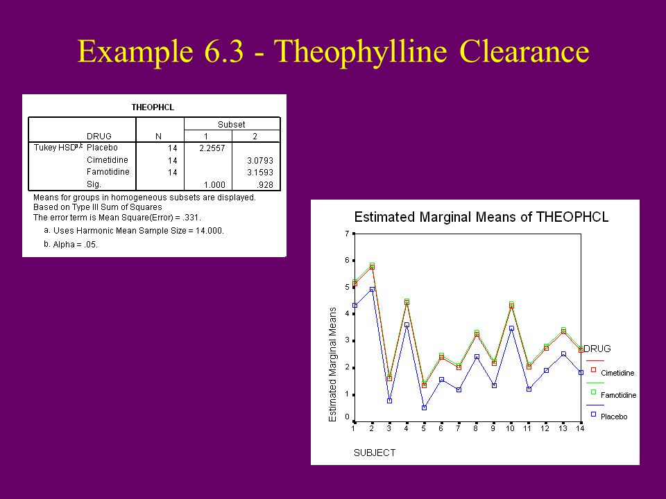
Randomized Block Design - F-test After Importing your dataset, and providing names to variables, click on: ANALYZE GENERAL LINEAR MODEL UNIVARIATE Assign the DEPENDENT VARIABLE Assign the TREATMENT variable as a FIXED FACTOR Assign the BLOCK variable as a RANDOM FACTOR Click on MODEL, then CUSTOM, under BUILD TERMS choose MAIN EFFECTS, move both factors to MODEL list Click on POST HOC and select the TREATMENT factor for POST HOC TESTS and BONFERRONI and TUKEY (among many choices) For PLOTS, Select the BLOCK factor for HORIZONTAL AXIS and the TREATMENT factor for SEPARATE LINES, click ADD
 For PLOTS, Select the BLOCK factor for HORIZONTAL AXIS and the TREATMENT factor for SEPARATE LINES, click ADD")
52
Example 6.3 - Theophylline Clearance

54
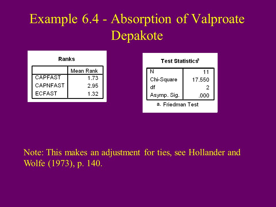
Randomized Block Design - Friedman’s test After Importing your dataset, and providing names to variables, click on: ANALYZE NONPARAMETRIC TESTS k RELATED SAMPLES For TEST VARIABLES, select the variables representing the treatments (each line is a subject/block) Click on FRIEDMAN
 Click on FRIEDMAN")
55
Example 6.4 - Absorption of Valproate Depakote Note: This makes an adjustment for ties, see Hollander and Wolfe (1973), p. 140.
56
2-Way ANOVA After Importing your dataset, and providing names to variables, click on: ANALYZE GENERAL LINEAR MODEL UNIVARIATE Assign the DEPENDENT VARIABLE Assign the FACTOR A variable as a FIXED FACTOR Assign the FACTOR B variable as a FIXED FACTOR Click on MODEL, then CUSTOM, select FULL FACTORIAL Click on POST HOC and select the both factors for POST HOC TESTS and BONFERRONI and TUKEY (among many choices) For PLOTS, Select FACTOR B for HORIZONTAL AXIS and FACTOR A for SEPARATE LINES, click ADD
 For PLOTS, Select FACTOR B for HORIZONTAL AXIS and FACTOR A for SEPARATE LINES, click ADD")
57
Example 6.5 - Nortriptyline Clearance

58
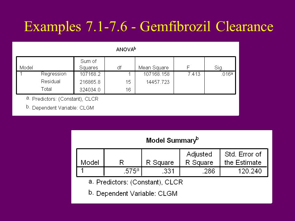
Linear Regression After Importing your dataset, and providing names to variables, click on: ANALYZE REGRESSION LINEAR Select the DEPENDENT VARIABLE Select the INDEPENDENT VARAIABLE(S) Click on STATISTICS, then ESTIMATES, CONFIDENCE INTERVALS, MODEL FIT For histogram of residuals, click on PLOTS, and HISTOGRAM under STANDARDIZED RESIDUAL PLOTS
 Click on STATISTICS, then ESTIMATES, CONFIDENCE INTERVALS, MODEL FIT For histogram of residuals, click on PLOTS, and HISTOGRAM under STANDARDIZED RESIDUAL PLOTS")
59
Examples 7.1-7.6 - Gemfibrozil Clearance

61
Example 7.8 - TB/Thalidomide in HIV

62
Useful Regression Plots Scatterplot with Fitted (Least Squares) Line –GRAPHS INTERACTIVE SCATTERPLOT –Select DEPENDENT VARIABLE for UP/DOWN AXIS –Select INDEPENDENT VARIABLE for RIGHT/LEFT AXIS –Click on FIT Tab, then REGRESSION for METHOD –NOTE: Be certain both variables are SCALE in VARIABLE VIEW under MEASURE Partial Regression Plots (Multiple Regression) to observe association of each Independent Variable with Y, controlling for all others –Fit REGRESSION model with all Independent Variables –Click PLOTS, then PRODUCE ALL PARTIAL PLOTS
 Line –GRAPHS INTERACTIVE SCATTERPLOT –Select DEPENDENT VARIABLE for UP/DOWN AXIS –Select INDEPENDENT VARIABLE for RIGHT/LEFT AXIS –Click on FIT Tab, then REGRESSION for METHOD –NOTE: Be certain both variables are SCALE in VARIABLE VIEW under MEASURE Partial Regression Plots (Multiple Regression) to observe association of each Independent Variable with Y, controlling for all others –Fit REGRESSION model with all Independent Variables –Click PLOTS, then PRODUCE ALL PARTIAL PLOTS")
63
Example 7.1 - Gemfibrozil Scatterplot

64
Logistic Regression After Importing your dataset, and providing names to variables, click on: ANALYZE REGRESSION BINARY LOGISTIC Select the DEPENDENT VARIABLE Select the INDEPENDENT VARAIABLE(S) as COVARIATES For a 95% CI for the odds ratio, click on OPTIONS, then CI for exp(B) Declare any CATEGORICAL COVARIATES (Independent variables whose levels are categorical, not numeric)
 as COVARIATES For a 95% CI for the odds ratio, click on OPTIONS, then CI for exp(B) Declare any CATEGORICAL COVARIATES (Independent variables whose levels are categorical, not numeric)")
65
Example 8.1 - Navelbine Toxicity Omnibus test for all regression coefficients (like F in linear regression)
")
66
Example 8.2 - CHD, BP, Cholesterol

67
Nonlinear Regression After Importing your dataset, and providing names to variables, click on: ANALYZE REGRESSION NONLINEAR Select the DEPENDENT VARIABLE Define the MODEL EXPRESSION as a function of the INDEPENDENT VARIABLE(s) and unknown PARAMETERS Define the PARAMETERS and give them STARTING VALUES (this may take several attempts)
 and unknown PARAMETERS Define the PARAMETERS and give them STARTING VALUES (this may take several attempts)")
68
Example 8.3 - MK-639 in AIDS Patients Nonlinear Regression Summary Statistics Dependent Variable RNACHNG Source DF Sum of Squares Mean Square Regression 3 24.97099 8.32366 Residual 2.02783.01391 Uncorrected Total 5 24.99881 (Corrected Total) 4 10.83973 R squared = 1 - Residual SS / Corrected SS =.99743 Asymptotic 95 % Asymptotic Confidence Interval Parameter Estimate Std. Error Lower Upper A 3.521788512.121466117 2.999161991 4.044415032 B 35.598069675 7.532265897 3.189345253 68.006794097 C 18374.392967 82.899219276 18017.706415 18731.079519

69
Survival Analysis -Kaplan-Meier Estimates and Log-Rank Test After Importing your dataset, and providing names to variables, click on: ANALYZE SURVIVAL KAPLAN-MEIER Select the variable representing the survival TIME of individual Select the variable representing the STATUS of individual (whether or not event has occured). NOTE: If the variable is an indicator that the observation was CENSORED, then a value of 0 for that variable will mean the event has occured. Select the variable representing the FACTOR containing the groups to be compared Click on COMPARE FACTOR, select LOG-RANK, and POOL ACROSS STRATA

70
Examples 9.1-2 - Navelbine and Taxol in Mice Survival Analysis for TIME Factor REGIMEN = 1 Time Status Cumulative Standard Cumulative Number Survival Error Events Remaining 6 0.9796.0202 1 48 8 0.9592.0283 2 47 22 0.9388.0342 3 46 32 0 4 45 32 0.8980.0432 5 44 35 0.8776.0468 6 43 41 0.8571.0500 7 42 46 0.8367.0528 8 41 54 0.8163.0553 9 40 Factor REGIMEN = 2 Time Status Cumulative Standard Cumulative Number Survival Error Events Remaining 8 0.9333.0644 1 14 10 0.8667.0878 2 13 27 0.8000.1033 3 12 31 0.7333.1142 4 11 34 0.6667.1217 5 10 35 0.6000.1265 6 9 39 0.5333.1288 7 8 47 0.4667.1288 8 7 57 0.4000.1265 9 6

71
Examples 9.1-2 - Navelbine and Taxol in Mice Test Statistics for Equality of Survival Distributions for REGIMEN Statistic df Significance Log Rank 10.93 1.0009 This is the square of the Z-statistic in text, and is a chi-square statistic

72
Relative Risk Regression (Cox Model) After Importing your dataset, and providing names to variables, click on: ANALYZE SURVIVAL COX REGRESSION Select the variable representing the survival TIME of individual Select the variable representing the STATUS of individual (whether or not event has occured). NOTE: If the variable is an indicator that the observation was CENSORED, then a value of 0 for that variable will mean the event has occured. Select the variable(s) representing the COVARIATES (Independent Variables in Model) Identify any CATEGORICAL COVARIATES including Dummy/Indicator variables K-M PLOTS can be obtained, with separate SURVIVAL curves by categories
 representing the COVARIATES (Independent Variables in Model) Identify any CATEGORICAL COVARIATES including Dummy/Indicator variables K-M PLOTS can be obtained, with separate SURVIVAL curves by categories.")
73
Example 9.3 - 6MP vs Placebo

Similar presentations
-the General Linear Model (GLM)>")
 Getting Started Guide.>")


 Lecture 10. Normality Check Frequency histogram (Skewness & Kurtosis) Probability plot, K-S test Normality Check Frequency histogram.>")


 18.0 WINDOWS.>")


