1. Analysis of variance (2) Lecture 10

2. Normality Check Frequency histogram (Skewness & Kurtosis) Probability plot, K-S test Normality Check Frequency histogram (Skewness & Kurtosis) Probability plot, K-S test Descriptive statistics Measurements (data) Measurements (data) Mean, SD, SEM, 95% confidence interval YES Check the Homogeneity of Variance Data transformation NO Data transformation NO Median, range, Q1 and Q3 Non-Parametric Test(s) For 2 samples: Mann- Whitney For 2-paired samples: Wilcoxon For >2 samples: Kruskal-Wallis Sheirer-Ray-Hare Non-Parametric Test(s) For 2 samples: Mann- Whitney For 2-paired samples: Wilcoxon For >2 samples: Kruskal-Wallis Sheirer-Ray-Hare Parametric Tests Student’s t tests for 2 samples; ANOVA for  2 samples; post hoc tests for multiple comparison of means Parametric Tests Student’s t tests for 2 samples; ANOVA for  2 samples; post hoc tests for multiple comparison of means YES One-way ANOVA Tukey’s test Two-way ANOVA F max test K-W test, Dunn’s test

3. Kruskal-Wallis test with tied ranks Example 10.11 (Zar, 1999) – comparison of pH among 4 ponds N = 8 + 8 + 7 + 8 = 31 H = {12/[N(N + 1)]}  (R i 2 /n i ) - 3(N + 1) H = {12/[31(31 + 1)]} (8917.8) - 3(31 + 1) = 11.876 Number of groups of tied ranks = m = 7  T =  (t i 3 - t i ) = (2 3 - 2) + (3 3 - 3) + (3 3 - 3) + (4 3 - 4) + (3 3 - 3) + (2 3 - 2) + (3 3 - 3) = 168 C = 1 -  T / (N 3 - N) = 1 - (168/ (31 3 - 31)) =0.9944 H c = H/C = 11.876/ 0.9944 = 11.943 = k - 1 = 4 -1 = 3  2 0.05, 3 = 7.815 < 11.943, 0.005< p <0.01, hence reject Ho (Table B1)

4. Dunn’s test is a non-parametric test and is used to compare any significant different means or medians. Using Example 10.11:  T = 168 For n A = 8 and n B = 8, SE =  {[(N(N + 1)/12) –  T /(12(N – 1)][(1/n A ) + (1/n B )]} SE =  {[(31(32)/12) – 168 /(12(31 – 1)][(1/8) + (1/8)]} = 4.53 For n A = 7 and n B = 8, SE =  {[(31(32)/12) – 168 /(12(31 – 1)][(1/7) + (1/8)]} = 4.69 Sample ranked by mean rank: 124 3 Rank sum:55132.5163.5145 Sample sizes:8887 Mean ranks:6.8816.5620.4420.71 Nonparametric multiple comparisons: Dunn’s test (e.g. 11.10, Zar 1999) In conclusion, water pH is the same in ponds 4 & 3 but is different in pond 1, and the relationship of pond 2 to the others is unclear. (see Table B15 for critical Q values) Similar to Tukey’s test

5. Normality Check Frequency histogram (Skewness & Kurtosis) Probability plot, K-S test Normality Check Frequency histogram (Skewness & Kurtosis) Probability plot, K-S test Descriptive statistics Measurements (data) Measurements (data) Mean, SD, SEM, 95% confidence interval YES Check the Homogeneity of Variance Data transformation NO Data transformation NO Median, range, Q1 and Q3 Non-Parametric Test(s) For 2 samples: Mann- Whitney For 2-paired samples: Wilcoxon For >2 samples: Kruskal-Wallis Sheirer-Ray-Hare Non-Parametric Test(s) For 2 samples: Mann- Whitney For 2-paired samples: Wilcoxon For >2 samples: Kruskal-Wallis Sheirer-Ray-Hare Parametric Tests Student’s t tests for 2 samples; ANOVA for  2 samples; post hoc tests for multiple comparison of means Parametric Tests Student’s t tests for 2 samples; ANOVA for  2 samples; post hoc tests for multiple comparison of means YES One-way ANOVA Tukey’s test Two-way ANOVA F max test K-W test, Dunn’s test Friedman Next lecture Other ANOVAs

6. Two-factor ANOVA 2-way ANOVA Can simultaneously assess the effects of two factors on a variable. Can also test for interaction among factors, provided that data in each cell of a contingency table consist observations n > 1. Assumption: normal data with equal variances but ANOVA is robust (see p. 185- 188, Zar 1999)

7. 2-way ANOVA with equal replication Example 12.1: The effects of sex and hormone treatment on plasma calcium concentrations (in mg/100 ml) of birds. Questions: Is there a significant difference between the mean calcium concentration of males and females? Is there a significant difference between the mean calcium concentration in each treatment (control vs. hormone treatment)?

8. Mean & 95% C.I.

9. Mean and 95% C.I. Two factors -Sex -Hormone F-Test Two-Sample for Variances Variable 1Variable 2 Mean32.5227.78 Variance69.71711.182 Observations55 df44 F6.234752 P(F<=f) one-tail0.052034 F Critical one-tail6.388233 Passed the Fmax test, indicating equal variances among the four means

10. SS total = SS within cells + SS between A + SS between B + SS interaction SS within cells = SS total – SS cells SS interaction = SS cells – SS between A – SS between B DF total = N – 1 DF cells (explained) = (n A )(n B ) – 1 DF within cells (residual or error) = (n A )(n B )(n’ – 1) where n’= no. of replicates within each cell DF between A = n A – 1 DF between B = n B – 1 DF A  B interaction = (DF between A )(DF between B )

11. SS total = 11354.3 – (436.5) 2 /20 = 1827.7 DF total = 20 – 1 = 19 SS cells = [(74.4) 2 + (60.6) 2 + (162.6) 2 + (138.9) 2 ]/5 - (436.5) 2 /20 = 1461.3 DF cells = (2)(2) - 1 = 3 SS within cells = SS total - SS cells = 1827.7 – 1461.3 = 366.4 DF within cells = (2)(2)(5 – 1) = 16

12. SS total = 11354.3 – (436.5) 2 /20 = 1827.7 DF total = 20 – 1 = 19 SS cells = [(74.4) 2 + (60.6) 2 + (162.6) 2 + (138.9) 2 ]/5 - (436.5) 2 /20 = 1461.3 DF cells = (2)(2) - 1 = 3 SS within cells = 1827.7 – 1461.3 = 366.4 DF within cells = (2)(2)(5 – 1) = 16 SS between treatments = {[(135.0) 2 + (301.5) 2 ] /(2)(5)} - (436.5) 2 /20 = 1386.1 DF between treatment = 2 - 1 = 1 SS between sexes = {[(237.0) 2 + (199.5) 2 ] /(2)(5)} - (436.5) 2 /20 = 70.31 DF between sexes = 2 - 1 = 1 SS interaction = SS cells – SS between A – SS between B = 1461.3 – 1386.1 – 70.31 = 4.900 DF interaction = (1)(1) = 1 Equations: See p. 242 (Zar, 1999)

13. Analysis of Variance Summary Table There was a significant effect of hormone treatment on plasma calcium concentrations in the birds (P <0.001). There was no interaction between sex and hormone treatment while the sex effect was not significant (likely due to inadequate power) Tukey test same as 1-way ANOVA

14. ANOVA Source of VariationSSdfMSFP-valueF crit Sample1386.1131 60.534<0.0014.494 Columns70.3131 3.0710.0994.494 Interaction4.9011 0.2140.6504.494 Within366.3721622.898 Total1827.69819 Output from Excel

15. [Ca] female male [Ca] control hormone treated control hormone treated [Ca] control hormone treated [Ca] control hormone treated Sex  Horm.  Sex X Horm.  Sex X Horm. X Sex  Horm. X

16. [Ca] female male [Ca] control hormone treated control hormone treated [Ca] control hormone treated [Ca] control hormone treated Sex  Horm.  Sex  Horm.  Intera.  Sex  Horm.  Intera.  Sex  Horm.  Intera. 

17. Interactive effects between variables: (a) no interaction; (b) interaction. (a) (b)

18. An example: The effects of light and sex on food intake in starlings. Total food intake (g) for 7 days

19. An example: The effects of light and sex on food intake in starlings. Two sexes have different food intake levels (p < 0.001). A significant interaction (p <0.05) indicates that two sexes respond significantly differently to day- length in the amount of food they eat.

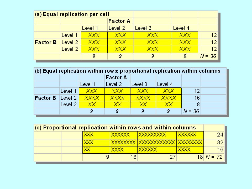
20. Computation of the F statistics for tests of significance in 2- way ANOVA with replicates

22. Cannot test for the interacting effect !

23. 2-way ANOVA for data without replication Interaction cannot be measured where data in each cell of a contingency table consist of single observations. Variability due to interaction is combined with the within variability and it is assumed to be negligible.

24. Other two experimental design suitable for 2-way ANOVA The randomized block See Example 12.4 (Zar, 99) Each block contains 4 animals: The randomized block See Example 12.4 (Zar, 99) Each block contains 4 animals: Repeated-measures See Example 12.5 (Zar, 1999) e.g. effects of diet type on food wastage in fish farm Repeated-measures See Example 12.5 (Zar, 1999) e.g. effects of diet type on food wastage in fish farm Other example: different colours of buckets (water traps) to sample insects Equivalent non-parametric method: Friedman’s analysis of variance by ranks (see p. 263-266, Zar 1999)

25. Use SPSS to conduct a 2-way ANOVA Column 1Column 2 Column 3 obs. 1 11 obs. 2 12 obs. 3 13 obs. i - 2 21 obs. i - 1 22 obs. i 23 Factor AFactor BDependent variable ……..

26. Normality Check Frequency histogram (Skewness & Kurtosis) Probability plot, K-S test Normality Check Frequency histogram (Skewness & Kurtosis) Probability plot, K-S test Descriptive statistics Measurements (data) Measurements (data) Mean, SD, SEM, 95% confidence interval YES Check the Homogeneity of Variance Data transformation NO Data transformation NO Median, range, Q1 and Q3 Non-Parametric Test(s) For 2 samples: Mann- Whitney For 2-paired samples: Wilcoxon For >2 samples: Kruskal-Wallis Sheirer-Ray-Hare Non-Parametric Test(s) For 2 samples: Mann- Whitney For 2-paired samples: Wilcoxon For >2 samples: Kruskal-Wallis Sheirer-Ray-Hare Parametric Tests Student’s t tests for 2 samples; ANOVA for  2 samples; post hoc tests for multiple comparison of means Parametric Tests Student’s t tests for 2 samples; ANOVA for  2 samples; post hoc tests for multiple comparison of means YES One-way ANOVA Tukey’s test Two-way ANOVA F max test K-W test, Dunn’s test Friedman Next lecture Other ANOVAs

27. Key notes After performing a Kruskal-Wallis test, a Dunn’s test can be used to identify any significantly different medians (or means) based on ranking Two-way ANOVA can be used to analyze samples which have been subjected to two levels of treatment In two-way ANOVA, there are several different design: (Model 1) both factors A and B are fixed factors; (Model 2) both factors are random factors; (Model 3) mixed factors. Furthermore, two-way ANOVA can also be applied to data with randomized block or repeated measure designs as well as data without replication. In two-way ANOVA, interaction cannot be tested where data in each cell of a contingency table consist of single observations.