1. CIS 601 Image ENHANCEMENT in the SPATIAL DOMAIN Dr. Rolf Lakaemper

2. Most of these slides base on the book Digital Image Processing by Gonzales/Woods

3. Spatial Filtering

4. Spatial Filtering: Operation on the set of ‘neighborhoods’ N(x,y) of each pixel 6820 122002010 226 68 12200 (Operator: sum)

5. Spatial Filtering Neighborhood of a pixel p at position x,y is a set N(p) of pixels defined relative to p. Example 1: N(p) = {(x,y): |x-x P |=1, |y-y P | = 1} P Q

6. Spatial Filtering More examples of neighborhoods: PPPP PP

7. Spatial Filtering Usually neighborhoods are used which are close to discs, since properties of the eucledian metric are often useful. The most prominent neighborhoods are the 4-Neighborhood and the 8-Neighborhood PP

8. Spatial Filtering We will define spatial filters on the 8-Neighborhood and their bigger relatives P P P N8 N24 N48

9. Spatial Filtering Index system for N8: n3n2n1 n6n5n4 n9n8n7

10. Spatial Filtering Motivation: what happens to P if we apply the following formula: P =  i n i n3n2n1 n6n5=Pn4 n9n8n7

11. Spatial Filtering What happens to P if we apply this formula: P =  i a i n i with a i given by: a3=1a2=1a1=1 a6=1a5=4a4=1 a9=1a8=1a7=1

12. Spatial Filtering Linear Image Filters Linear operations calculate the resulting value in the output image pixel f(i,j) as a linear combination of brightness in a local neighborhood of the pixel h(i,j) in the input image. This equation is called discrete convolution: Function w is called a convolution kernel or a filter mask. In our case it is a rectangle of size (2a+1)x(2b+1).

13. Spatial Filtering

14. Exercise: Compute the 2-D linear convolution of signal X with mask w. Extend the signal X with 0’s if needed (padding).

15. Spatial Filtering Lets have a look at different values of a i and their effects ! This MATLAB program creates an interesting output: % Description: given an image 'im', % create 12 filtered versions using % randomly designed filters for i=1:12 a=rand(7,7); % create a % random 7x7 % filter-matrix a=a*2 - 1; % range: -1 to 1 a=a/sum(a(:)); % normalize im1=conv2(im,a);% Filter subplot(4,3,i); imshow(im1/max(im1(:))); end

16. Spatial Filtering

17. Different effects of the previous slides included: Blurring / Smoothing Sharpening Edge Detection All these effects can be achieved using different coefficients.

18. Spatial Filtering Blurring / Smoothing (Sometimes also referred to as averaging or lowpass-filtering) Average the values of the center pixel and its neighbors: Purpose: Reduction of ‘irrelevant’ details Noise reduction Reduction of ‘false contours’ (e.g. produced by zooming)

19. Spatial Filtering Blurring / Smoothing 111 111 111 * 1/9 Apply this scheme to every single pixel !

20. Spatial Filtering Example 2: Weighted average 121 242 121 * 1/16

21. Spatial Filtering Basic idea: Weigh the center point the highest, decrease weight by distance to center. The general formula for weighted average: P =  i a i n i /  i a i Constant value, depending on mask, not on image !

22. Spatial Filtering Blurring using different radii (=size of neighborhood)

23. Spatial Filtering EDGE DETECTION

24. Spatial Filtering EDGE DETECTION Purpose: Preprocessing Sharpening

25. Spatial Filtering What are edges in an image? " Edges are those places in an image that correspond to object boundaries. " Edges are pixels where image brightness changes abruptly. Brightness vs. Spatial Coordinates

26. Spatial Filtering Motivation: Derivatives

27. Spatial Filtering First and second order derivative

28. Spatial Filtering First and second order derivative 1. 1 st order generally produces thicker edges 2. 2 nd order shows stronger response to detail 3. 1 st order generally response stronger to gray level step 4. 2 nd order produce double (pos/neg) response at step change

29. Spatial Filtering Definition of 1 dimensional discrete 1 st order derivative: dF/dX = f(x+1) – f(x) The 2 nd order derivative is the derivative of the 1 st order derivative…

30. Spatial Filtering The 2 nd order derivative is the derivative of the 1 st order derivative… F(x-1)F(x)F(x+1) F(x)-F(x-1)F(x+1)-F(x)F(x+2)-F(x+1) derive F(x+1)-F(x) – (F(x)-F(x-1)) F(x+1)-F(x) – (F(x)-F(x-1))= F(x+1) -2F(x)+F(x-1)

31. Spatial Filtering F(x+1)-F(x) – (F(x)-F(x-1))= F(x+1) -2F(x) +F(x-1) 1-21 One dimensional 2 nd derivative in x direction: One dimensional 2 nd derivative, direction y: -2 1 1

32. Spatial Filtering 1-21 TWO dimensional 2 nd derivative (derivatives are linear !): -2 1 1 + = 000 0000 0 0 0 0 0 -4 1 1 0 1 0 0 1 0 This mask is called the ‘LAPLACIAN’ (remember calculus ?)

33. Spatial Filtering Different variants of the Laplacian

34. Spatial Filtering Effect of the Laplacian… (MATLAB) im = im/max(im(:)); % create laplacian L=[1 1 1;1 -8 1; 1 1 1]; % Filter ! im1=conv2(im,L); % normalize and show im1=(im1-min(im1(:))) / (max(im1(:))-min(im1(:))); imshow(im1);

35. Spatial Filtering

36. A Quick Note " Matlab’s image processing toolbox provides edge function to find edges in an image: I = imread('rice.tif'); BW1 = edge(I,'prewitt'); BW2 = edge(I,'canny'); imshow(BW1) figure, imshow(BW2) " Edge function supports six different edge- finding methods: Sobel, Prewitt, Roberts, Laplacian of Gaussian, Zero-cross, and Canny.

37. Spatial Filtering Edges detected by the Laplacian can be used to sharpen the image ! +

38. Spatial Filtering

39. Sharpening can be done in 1 pass: 4 1 0 0 + = 0 0 0 00 0 0 0 0 0 5 0 0 0 0 LAPLACIANOriginal ImageSharpened Image

40. Spatial Filtering Sharpening in General: Unsharp Masking and High Boost Filtering

41. Spatial Filtering Basic Idea (unsharp masking): Subtract a BLURRED version of an image from the image itself ! F sharp = F – F blurred

42. Spatial Filtering Variation: emphasize original image (high-boost filtering): F sharp = a*F – F blurred, a>=1 0a01 1 1 - = 000 0000 1 0 0 1 0 a-1 0 0 0 0

43. Spatial Filtering Different Examples of High-Boost Filters: 0 0 0 0 0 a=1 5 0 0 0 0 a=6 1e7 0 0 0 0 a=1e7+1 Laplacian + Image !

44. Spatial Filtering

45. Enhancement using the First Derivative: The Gradient Definition: 2 dim. column vector,  (f) = [G x ; G y ], G is 1 st order derivative MAGNITUDE of gradient: Mag(  (f))= SQRT(G x 2 + G y 2 )

46. Spatial Filtering For computational reasons the magnitude is often approximated by: Mag ~ abs(G x ) + abs(G y )

47. Spatial Filtering Mag ~ abs(G x ) + abs(G y ) 0 -2 2 0 1 0 1 0 0 0 1 2 1 -2 “Sobel Operators”

48. Spatial Filtering Sobel Operators are a pair of operators ! Effect of Sobel Filtering:

49. Spatial Filtering Sobel Operators are a pair of operators !

50. Spatial Filtering Remember the result some slides ago: First and second order derivative 1. 1 st order generally produces thicker edges 2. 2 nd order shows stronger response to detail 3. 1 st order generally response stronger to gray level step 4. 2 nd order produce double (pos/neg) response at step change

51. Spatial Filtering In practice, multiple filters are combined to enhance images

52. Spatial Filtering …continued

53. Spatial Filtering

54. Non – Linear Filtering: Order-Statistics Filters Median Min Max

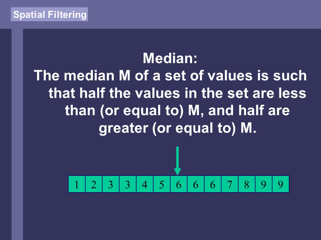
55. Spatial Filtering Median: The median M of a set of values is such that half the values in the set are less than (or equal to) M, and half are greater (or equal to) M. 1233456667899

56. Spatial Filtering Most important properties of the median: less sensible to noise than mean an element of the original set of values Can be computed in O(n)

57. Spatial Filtering Median vs. Mean

58. Spatial Filtering Min and Max 4 5 4 7 2 8 2 3 3 3 3 3 3333 MIN MAX 2 5 4 7 2 8 2 3 3 3 3 3 3333 8 5 4 7 2 8 2 3 3 3 3 3 3333

59. Spatial Filtering Basics of Morphological Filtering

60. Spatial Filtering Dilation:

61. Spatial Filtering Erosion:

62. Spatial Filtering opening:

63. Spatial Filtering closing:

64. Spatial Filtering Opening on binary images: for i=2:2:18 se = strel('disk',i); imo = imopen(im1,se); subplot(3,3,(i)/2); imshow(imo); s=sprintf('disksize: %d',i); title(s); end

65. Spatial Filtering Opening on gray images:

66. Spatial Filtering Closing on binary images: for i=2:2:18 se = strel('disk',i); imo = imclose(im1,se); subplot(3,3,(i)/2); imshow(imo); s=sprintf('disksize: %d',i); title(s); end

67. Spatial Filtering Closing on gray images:

68. Spatial Filtering Closing o Opening & Opening o Closing

69. Spatial Filtering Morphological Edges: Dilation - Original

70. Spatial Filtering (Exercise: surveillance camera)

71. Spatial Filtering …end of Operations in Spatial Domain. And now to something completely different ( really ?)

72. The FREQUENCY Domain

73. Some of these slides base on the textbook Digital Image Processing by Gonzales/Woods Chapter 4

74. Frequency Domain So far we processed the image ‘directly’, i.e. the transformation was a function of the image itself. We called this the SPATIAL domain. So what’s the FREQUENCY domain ?

75. Sound Let’s first forget about images, and look at SOUND. SOUND: 1 dimensional function of changing (air-)pressure in time Pressure Time t

76. Sound SOUND: if the function is periodic, we perceive it as sound with a certain frequency (else it’s noise). The frequency defines the pitch. Pressure Time t

77. Sound The AMPLITUDE of the curve defines the VOLUME

78. Sound The SHAPE of the curve defines the sound character Flute String Brass

79. Sound How can the SHAPE of the curve be defined ?

80. Sound Listening to an orchestra, you can distinguish between different instruments, although the sound is a SINGLE FUNCTION ! Flute String Brass

81. Sound If the sound produced by an orchestra is the sum of different instruments, could it be possible that there are BASIC SOUNDS, that can be combined to produce every single sound ?

82. Sound The answer (Charles Fourier, 1822): Any function that periodically repeats itself can be expressed as the sum of sines/cosines of different frequencies, each multiplied by a different coefficient

83. Sound Or differently: Since a flute produces a sine-curve like sound, a (huge) group of (outstanding) talented flautists could replace a classical orchestra. (Don’t take this remark seriously, please)

84. 1D Functions A look at SINE / COSINE The sine-curve is defined by: Frequency (the number of oscillations between 0 and 2*PI) Amplitude (the height) Phase (the starting angle value) The constant y-offset, or DC (direct current)

85. 1D Functions The general sine-shaped function: f(t) = A * sin(  t +  ) + c Amplitude Frequency Phase Constant offset (usually set to 0)

86. 1D Functions Remember Fourier: …A function…can be expressed as the sum of sines/cosines… What happens if we add sine and cosine ?

87. 1D Functions a * sin(  t) + b * cos(  t) = A * sin(  t +  ) (with A=sqrt(a^2+b^2) and tan  = b/a)  Adding sine and cosine of the same frequency yields just another sine function with different phase and amplitude, but same frequency. Or: adding a cosine simply shifts the sine function left/right and stretches it in y-direction. It does NOT change the sine-character and frequency of the curve.

88. 1D Functions Remember Fourier, part II: Any function that periodically repeats itself… => To change the shape of the function, we must add sine-like functions with different frequencies.

89. 1D Functions This applet shows the result: Applet: Fourier Synthesis

90. 1D Functions What did we do ? Choose a sine curve having a certain frequency, called the base-frequency Choose sine curves having an integer multiple frequency of the base-frequency Shift each single one horizontally using the cosine-factor Choose the amplitude-ratio of each single frequency Sum them up

91. 1D Functions This technique is called the FOURIER SYNTHESIS, the parameters needed are the sine/cosine ratios of each frequency. The parameters are called the FOURIER COEFFICIENTS

92. 1D Functions As a formula: f(x)= a 0 /2 +  k=1..n a k cos(kx) + b k sin(kx) Fourier Coefficients

93. Note: The set of a k, b k TOTALLY defines the CURVE synthesized ! We can therefore describe the SHAPE of the curve or the CHARACTER of the sound by the (finite ?) set of FOURIER COEFFICIENTS ! 1D Functions

94. Examples for curves, expressed by the sum of sines/cosines (the FOURIER SERIES): 1D Functions

95. SAWTOOTH Function 1D Functions f(x) = ½ - 1/pi *  n 1/n *sin (n*pi*x) Freq.sincos 110 21/20 31/30 41/40

96. SQUARE WAVE Function 1D Functions f(x) = 4/pi *  n=1,3,5 1/n *sin (n*pi*x) Freq.sincos 110 31/30 51/50 71/70

97. What does the set of FOURIER COEFFICIENTS tell about the character of the shape ? 1D Functions

98. Result: Steep slopes introduce HIGH FREQUENCIES. 1D Functions

99. Motivation for Image Processing: Steep slopes showed areas of high contrast… …so it would be nice to be able to get the set of FOURIER COEFFICIENTS if an arbitrary (periodically) function is given. (So far we talked about 1D functions, not images, this was just a motivation) 1D Functions

100. The Problem now: Given an arbitrary but periodically 1D function (e.g. a sound), can you tell the FOURIER COEFFICIENTS to construct it ? 1D Functions

101. The answer (Charles Fourier): YES. 1D Functions

102. With: e ix =cos(x)+ i sin(x) The coefficients F(u) are given by (continous): F(u)=  f(x)e -i2  ux dx Discrete (M=number of samples): F(u)=1/M  x   f(x)e -i2  ux/M 1D Functions

103. Note the similarity between analysis and synthesis: Analysis : F(u)=1/M  x=0   f(x)e -i2  ux/M dx (with u=0..M-1) Synthesis: f(x)=  u=0..M-1  F(u)e i2  ux/M (with x=0..M-1) 1D Functions

104. We don’t want to explain the mathematics behind the answer here, but simply use the MATLAB Fourier Transformation Function. 1D Functions

105. MATLAB - function fft: Input: A vector, representing the discrete function Output: The Fourier Coefficients as vector of imaginary numbers, scaled 1D Functions

106. Example: 1D Functions x=0:2*pi/(2047):2*pi; s=sin(x)+cos(x) + sin(2*x) + 0.3*cos(2*x); f=fft(s); 1.31026.2 - 1022.8i 310.1 - 1022.1i -0.4 + 1.6i Freq. 0Freq. 1Freq. 2Freq. 3 cos sin

107. 1D Functions FrReIm 01.30 11026.21022.8 2310.11022.1 FrReIm 0~00 1~1 2~0.3~1 1.31026.2 - 1022.8i 310.1 - 1022.1i -0.4 + 1.6i Transformation: t(a) = 2*a / length(result vector)

108. 1D Functions The fourier coefficients are given by: F=fft(function) L=length(F); %this is always = length(function) Coefficient for cosine, frequency k-times the base frequency: real(F(k+1)) * 2 / L Coefficient for sine, frequency k-times the base frequency: imag(F(k+1)) * 2 / L Since: a * sin(  t) + b * cos(  t) = A * sin(  t +  ) the Amplitude is given by: A=sqrt(a^2+b^2), The Phase by: tan  = b/a

109. 1D Functions An application using the Fourier Transform: Create an autofocus system for a digital camera We did this already, but differently ! (MATLAB DEMO)

110. 1D Functions Second application: Shape Database using Fourier Features (revisited)

111. Some Results query Top 9

112. Some Results query Top 9

113. 2D Functions From Sound to Images: 2D Fourier Transform

114. 2D Functions The idea: Extend the base functions to 2 dimensions: f u (x) = sin(ux)  f u,v (x,y) = sin(ux + vy)

115. 2D Functions Some examples: The base function, direction x: u=1, v=0 y x

116. 2D Functions The base function, direction y: u=0, v=1

117. 2D Functions u=2, v=0

118. 2D Functions u=0, v=2

119. 2D Functions u=1, v=1

120. 2D Functions u=1, v=2

121. 2D Functions u=1, v=3

122. 2D Functions As in 1D, the 2D image can be phase-shifted by adding a weighted cosine function: f u,v (x,y) = a k sin(ux + vy) + b k cos(ux + vy) + =

123. 2D Functions As basic functions, we get a pair of sine/cosine functions for every pair of frequency-multiples (u,v): sin cos sin cos sin cos sin cos sin cos sin cos sin cos sin cos sin cos sin cos sin cos sin cos v u

124. 2D Functions Every single sin/cos function gets a weight, which is the Fourier Coefficient: a b a b a b a b v u a b a b a b a b a b a b a b a b

125. 2D Functions Summing all basic functions with their given weight gives a new function. As in 1D: Every 2D function can be synthesized using the basic functions with specific weights. As in 1D: The set of weights defines the 2D function.

126. 2D Functions Example: Summing basic functions of different frequencies:

127. 2D Functions Example: Summing basic functions of different frequencies:

128. 2D Functions MATLAB Demo: Bear Reconstruction