1. Project Management With PERT/CPM
A Case Study: The Reliable Construction Co. Project (Section 16.1)
Using a Network to Visually Display a Project (Section 16.2)
Scheduling a Project with PERT/CPM (Section 16.3)
Dealing with Uncertain Activity Durations (Section 16.4)
Considering Time-Cost Tradeoffs (Section 16.5)
Scheduling and Controlling Project Costs (Section 16.6)
McGraw-Hill/Irwin
Copyright © 2011 by the McGraw-Hill Companies, Inc. All rights reserved.

2. Reliable Construction Company Project
The Reliable Construction Company has just made the winning bid of $5.4 million to construct a new plant for a major manufacturer.
The contract includes the following provisions:
A penalty of $300,000 if Reliable has not completed construction within 47 weeks.
A bonus of $150,000 if Reliable has completed the plant within 40 weeks.
Questions:
How can the project be displayed graphically to better visualize the activities?
What is the total time required to complete the project if no delays occur?
When do the individual activities need to start and finish?
What are the critical bottleneck activities?
For other activities, how much delay can be tolerated?
What is the probability the project can be completed in 47 weeks?
What is the least expensive way to complete the project within 40 weeks?
How should ongoing costs be monitored to try to keep the project within budget?
16-2

3. Activity List for Reliable Construction
Activity Description
Immediate Predecessors
Estimated Duration (Weeks) A
Excavate — 2 B
Lay the foundation 4 C
Put up the rough wall 10 D
Put up the roof 6 E
Install the exterior plumbing F
Install the interior plumbing 5 G
Put up the exterior siding 7 H
Do the exterior painting
E, G 9 I
Do the electrical work J
Put up the wallboard
F, I 8 K
Install the flooring L
Do the interior painting M
Install the exterior fixtures N
Install the interior fixtures
K, L
Table Activity list for the Reliable Construction Co. project.
16-3

4. Project Networks
A network used to represent a project is called a project network.
A project network consists of a number of nodes and a number of arcs.
Two types of project networks:
Activity-on-arc (AOA): each activity is represented by an arc. A node is used to separate an activity from its predecessors. The sequencing of the arcs shows the precedence relationships.
Activity-on-node (AON): each activity is represented by a node. The arcs are used to show the precedence relationships.
Advantages of AON (used in this textbook):
considerably easier to construct
easier to understand
easier to revise when there are changes
16-4

5. Reliable Construction Project Network
Figure The project network for the Reliable Construction Co. project.
16-5

6. The Critical Path
A path through a network is one of the routes following the arrows (arcs) from the start node to the finish node.
The length of a path is the sum of the (estimated) durations of the activities on the path.
The (estimated) project duration equals the length of the longest path through the project network.
This longest path is called the critical path. (If more than one path tie for the longest, they all are critical paths.)
16-6

7. The Paths for Reliable’s Project Network
Length (Weeks)
StartA B C D G H M Finish
= 40
Start A B C E H M Finish
= 31
Start A B C E F J K N Finish
= 43
Start A B C E F J L N Finish
= 44
Start A B C I J K N Finish
= 41
Start A B C I J L N Finish
= 42
Table The paths and path lengths through Reliable’s Project Network.
16-7

8. Earliest Start and Earliest Finish Times
The starting and finishing times of each activity if no delays occur anywhere in the project are called the earliest start time and the earliest finish time.
ES = Earliest start time for a particular activity
EF = Earliest finish time for a particular activity
Earliest Start Time Rule: ES = Largest EF of the immediate predecessors.
Procedure for obtaining earliest times for all activities:
For each activity that starts the project (including the start node), set its ES = 0.
For each activity whose ES has just been obtained, calculate EF = ES + duration.
For each new activity whose immediate predecessors now have EF values, obtain its ES by applying the earliest start time rule. Apply step 2 to calculate EF.
Repeat step 3 until ES and EF have been obtained for all activities.
16-8

9. ES and EF Values for Reliable Construction for Activities that have only a Single Predecessor
Figure Earliest start time (ES) and earliest finish time (EF) values for the initial activities in Figure 16.1 that have only a single immediate predecessor.
16-9

10. ES and EF Times for Reliable Construction
Figure Earliest start time (ES) and earliest finish time (EF) values for all the activities (plus the start and finish nodes) of the Reliable Construction Co. project.
16-10

11. Latest Start and Latest Finish Times
The latest start time for an activity is the latest possible time that it can start without delaying the completion of the project (so the finish node still is reached at its earliest finish time). The latest finish time has the corresponding definition with respect to finishing the activity.
LS = Latest start time for a particular activity
LF = Latest finish time for a particular activity
Latest Finish Time Rule: LF = Smallest LS of the immediate successors.
Procedure for obtaining latest times for all activities:
For each of the activities that together complete the project (including the finish node), set LF equal to EF of the finish node.
For each activity whose LF value has just been obtained, calculate LS = LF –  duration.
For each new activity whose immediate successors now have LS values, obtain its LF by applying the latest finish time rule. Apply step 2 to calculate its LS.
Repeat step 3 until LF and LS have been obtained for all activities.
16-11

12. LS and LF Times for Reliable’s Project
Figure Latest start time (LS) and latest finish time (LF) for all the activities (plus the start and finish nodes) of the Reliable Construction Co. project.
16-12

13. The Complete Project Network
Figure The complete project network showing ES and LS (in the upper parentheses next to the node) and EF and LF (in the lower parentheses next to the node) for each activity of the Reliable Construction Co. project. The darker arrows show the critical path through the project network.
16-13

14. Slack for Reliable’s Activities
Activity
Slack (LF–EF)
On Critical Path? A
Yes B C D 4 No E F G H I 2 J K 1 L M N
Table Slack for Reliable’s activities.
16-14

15. Spreadsheet to Calculate ES, EF, LS, LF, Slack
Figure A spreadsheet to calculate the ES, EF, LS, LF, slack, and whether or not it is critical, for each activity in Reliable Construction Co.’s project network.
16-15

16. The PERT Three Estimate Approach
Most likely estimate (m) = Estimate of most likely value of the duration Optimistic estimate (o) = Estimate of duration under most favorable conditions. Pessimistic estimate (p) = Estimate of duration under most unfavorable conditions.
Figure Model of the probability distribution of the duration of an activity for the PERT three-estimate approach: m = most likely estimate, o = optimistic estimate, p = pessimistic estimate.
16-16

17. Mean and Standard Deviation
An approximate formula for the variance (2) of an activity is
An approximate formula for the mean (m) of an activity is
16-17

18. Time Estimates for Reliable’s Project
Activity o m p
Mean
Variance A 1 2 3
1/9 B
3.5 8 4 C 6 9 18 10 D
5.5 E
4.5 5
4/9 F G
6.5 11 7 H 17 I
7.5 J K L M N
Table Expected value and variance of the duration of each activity for Reliable’s project
16-18

19. Pessimistic Path Lengths for Reliable’s Project
Pessimistic Length (Weeks)
StartA B C D G H M Finish
= 70
Start A B C E H M Finish
= 54
Start A B C E F J K N Finish
= 66
Start A B C E F J L N Finish
= 69
Start A B C I J K N Finish
= 60
Start A B C I J L N Finish
= 63
Table The paths and path lengths through Reliable’s project network when the duration of each activity equals its pessimistic estimate.
16-19

20. Three Simplifying Approximations of PERT/CPM
The mean critical path will turn out to be the longest path through the project network.
The durations of the activities on the mean critical path are statistically independent. Thus, the three estimates of the duration of an activity would never change after learning the durations of some of the other activities.
The form of the probability distribution of project duration is the normal distribution. By using simplifying approximations 1 and 2, there is some statistical theory (one version of the central limit theorem) that justifies this as being a reasonable approximation if the number of activities on the mean critical path is not too small.
16-20

21. Calculation of Project Mean and Variance
Activities on Mean Critical Path
Mean
Variance A 2
1/9 B 4 1 C 10 E
4/9 F 5 J 8 L N 6
Project duration
mp = 44
s2p = 9
Table Calculation of mp and s2p for Reliable’s project.
16-21

22. Probability of Meeting Deadline
Figure The three simplifying approximations lead to the probability distribution of the duration of Reliable’s project being approximated by the normal distribution shown here. The shaded area is the portion of the distribution that meets the deadline of 47 weeks.
16-22

23. Probability of Meeting a Deadline
P(T ≤ d)
P(T ≤ d)
–3.0
0.0014
0.50
–2.5
0.0062
0.25
0.60
–2.0
0.023
0.5
0.69
–1.75
0.040
0.75
0.77
–1.5
0.067
1.0
0.84
–1.25
0.11
1.25
0.89
–1.0
0.16
1.5
0.933
–0.75
0.23
1.75
0.960
–0.5
0.31
2.0
0.977
–0.25
0.40
2.5
0.9938
3.0
0.9986
Table Approximate probability of meeting a project deadline.
16-23

24. Spreadsheet for PERT Three-Estimate Approach
Figure This Excel template in your MS Courseware enables efficient application of the PERT three-estimate approach, as illustrated here for Reliable’s project.
16-24

25. Considering Time-Cost Trade-Offs
Question: If extra money is spent to expedite the project, what is the least expensive way of attempting to meet the target completion time (40 weeks)?
CPM Method of Time-Cost Trade-Offs:
Crashing an activity refers to taking special costly measures to reduce the duration of an activity below its normal value. Special measures might include overtime, hiring additional temporary help, using special time-saving materials, obtaining special equipment, etc.
Crashing the project refers to crashing a number of activities to reduce the duration of the project below its normal value.
16-25

26. Time-Cost Graph for an Activity
Figure A typical time-cost graph for an activity.
16-26

27. Time-Cost Trade-Off Data for Reliable’s Project
  Time (weeks)  
             Cost             
Maximum Reduction in Time (weeks)
Crash Cost per Week Saved
Activity
Normal
Crash A 2 1
$180,000
$280,000
$100,000 B 4
320,000
420,000
50,000 C 10 7
620,000
860,000 3
80,000 D 6
260,000
340,000
40,000 E
410,000
570,000
160,000 F 5
180,000 G
900,000
1,020,000 H 9
200,000
380,000
60,000 I
210,000
270,000
30,000 J 8
430,000
490,000 K L
250,000
350,000 M
100,000 N
330,000
510,000
Table Time-Cost trade-off data for the activities of Reliable’s project.
16-27

28. Marginal Cost Analysis for Reliable’s Project Initial Table
Length of Path
Activity to Crash
Crash Cost
ABCDGHM
ABCEHM
ABCEFJKN
ABCEFJLN
ABCIJKN
ABCIJLN 40 31 43 44 41 42
Table The initial table for starting marginal cost analysis of Reliable’s project.
16-28

29. Marginal Cost Analysis for Reliable’s Project Table After Crashing One Week
Length of Path
Activity to Crash
Crash Cost
ABCDGHM
ABCEHM
ABCEFJKN
ABCEFJLN
ABCIJKN
ABCIJLN 40 31 43 44 41 42 J
$30,000
Marginal cost analysis of Reliable’s project. Activity J is the cheapest activity to crash on the critical path (ABCEFJLN).
16-29

30. Marginal Cost Analysis for Reliable’s Project Table After Crashing Two Weeks
Length of Path
Activity to Crash
Crash Cost
ABCDGHM
ABCEHM
ABCEFJKN
ABCEFJLN
ABCIJKN
ABCIJLN 40 31 43 44 41 42 J
$30,000 39
Marginal cost analysis of Reliable’s project. Activity J is still the cheapest activity to crash on the critical path (ABCEFJLN).
16-30

31. Marginal Cost Analysis for Reliable’s Project Table After Crashing Three Weeks
Length of Path
Activity to Crash
Crash Cost
ABCDGHM
ABCEHM
ABCEFJKN
ABCEFJLN
ABCIJKN
ABCIJLN 40 31 43 44 41 42 J
$30,000 39 F
$40,000
Marginal cost analysis of Reliable’s project. Activity F is now the cheapest activity to crash on the critical path (ABCEFJLN), since activity J has already been crashed as far as possible..
16-31

32. Marginal Cost Analysis for Reliable’s Project Final Table After Crashing Four Weeks
Length of Path
Activity to Crash
Crash Cost
ABCDGHM
ABCEHM
ABCEFJKN
ABCEFJLN
ABCIJKN
ABCIJLN 40 31 43 44 41 42 J
$30,000 39 F
$40,000
Table The final table for performing marginal cost analysis of Reliable’s project. Activity F is the cheapest activity to crash on the critical path (ABCEFJLN), since activity J has already been crashed as far as possible.
16-32

33. Project Network After Crashing
Figure The project network if activities J and F are fully crashed (with all other activities normal) for Reliable’s project. The darker arrows show the various critical paths through the project network.
16-33

34. Using LP to Make Crashing Decisions
Restatment of the problem: Consider the total cost of the project, including the extra cost of crashing activities. The problem then is to minimize this total cost, subject to the constraint that project duration must be less than or equal to the time desired by the project manager.
The decisions to be made are the following:
The start time of each activity.
The reduction in the duration of each activity due to crashing.
The finish time of the project (must not exceed 40 weeks).
The constraints are:
Time Reduction ≤ Max Reduction (for each activity).
Project Finish Time ≤ Desired Finish Time.
Activity Start Time ≥ Activity Finish Time of all predecessors (for each activity).
Project Finish Time ≥ Finish Time of all immediate predecessors of finish node.
16-34

35. Spreadsheet Model
Figure The spreadsheet displays the application of the CPM method of time-cost trade-offs to Reliable’s project, where columns I and J show the optimal solution obtained by using the Excel Solver.
16-35

36. Mr. Perty’s Conclusions
The plan for crashing the project only provides a 50 percent chance of actually finishing the project within 40 weeks, so the extra cost of the plan ($140,000) is not justified. Therefore, Mr. Perty rejects any crashing at this stage.
The extra cost of the crashing plan can be justified if it almost certainly would earn the bonus of $150,000 for finishing the project within 40 weeks. Therefore, Mr. Perty will hold the plan in reserve to be implemented if the project is running well ahead of schedule before reaching activity F.
The extra cost of part or all of the crashing plan can be easily justified if it likely would make the difference in avoiding the penalty of $300,000 for not finishing the project within 47 weeks. Therefore, Mr. Perty will hold the crashing plan in reserve to be partially or wholly implemented if the project is running far behind schedule before reaching activity F or activity J.
16-36

37. Scheduling and Controlling Project Costs
PERT/Cost is a systematic procedure (normally computerized) to help the project manager plan, schedule, and control costs.
Assumption: A common assumption when using PERT/Cost is that the costs of performing an activity are incurred at a constant rate throughout its duration.
16-37

38. Budget for Reliable’s Project
Activity
Estimated Duration (weeks)
Estimated Cost
Cost per Week of Its Duration A 2
$180,000
$90,000 B 4
320,000
80,000 C 10
620,000
62,000 D 6
260,000
43,333 E
410,000
102,500 F 5
180,000
36,000 G 7
900,000
128,571 H 9
200,000
22,222 I
210,000
30,000 J 8
430,000
53,750 K
160,000
40,000 L
250,000
50,000 M
100,000 N
330,000
55,000
Table The project budget for Reliable’s project.
16-38

39. PERT/Cost Spreadsheet (Earliest Start Times)
Figure This Excel template in your MS Courseware enables efficient application of the PERT/Cost procedure, as illustrated here for the beginning of Reliable’s project when using earliest start times.
16-39

40. PERT/Cost Spreadsheet (Earliest Start Times)
Figure This spreadsheet extends the template in Figure to weeks 17 to 25.
16-40

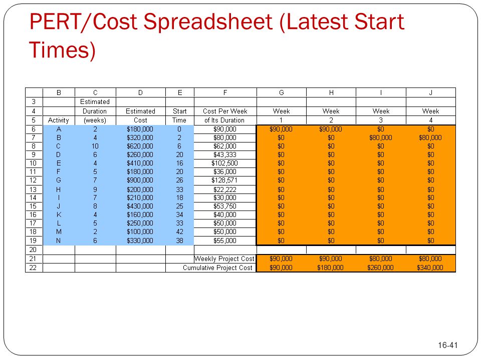
41. PERT/Cost Spreadsheet (Latest Start Times)
16-41

42. PERT/Cost Spreadsheet (Latest Start Times)
Figure The application of the PERT/Cost procedure to weeks 17 to 25 of Reliable’s project when using latest start times.
16-42

43. Cumulative Project Costs
Figure The schedule of cumulative project costs when all activities begin at their earliest start times (the top cost curve) or at their latest start times (the bottom cost curve).
16-43

44. PERT/Cost Report after Week 22
Activity
Budgeted Cost
Percent Completed
Value Completed
Actual Cost to Date
Cost Overrun to Date A
$180,000
100%
$200,000
$20,000 B
320,000
100
330,000
10,000 C
620,000
600,000
–20,000 D
260,000 75
195,000
200,000
5,000 E
410,000
400,000
–10,000 F
180,000 25
45,000
60,000
15,000 I
210,000 50
105,000
130,000
25,000
Total
$2,180,000
$1,875,000
$1,920,000
$45,000
Table PERT/Cost Report after Week 22 of Reliable’s project.
16-44