1. 7
Government Influences on Markets
CHAPTER
“If you put the federal government in charge of the Sahara Desert, in 5 years there'd be a shortage of sand.”
Milton Friedman
Nobel Laureate, Economics
(1912 – 2006)
Notes and teaching tips: 5, 7, 13, 32, 34, 35, 36, 52, and 53.
To view a full-screen figure during a class, click the red “expand” button.
To return to the previous slide, click the red “shrink” button.
To advance to the next slide, click anywhere on the full screen figure.

2. C H A P T E R C H E C K L I S T
When you have completed your study of this chapter, you will be able to
1 Explain how taxes change prices and quantities, are shared by buyers and sellers, and create inefficiency.
2 Explain how a price ceiling works and show how a rent ceiling creates a housing shortage, inefficiency, and unfairness.
3 Explain how a price floor works and show how the minimum wage creates unemployment, inefficiency, and unfairness.

3. C H A P T E R C H E C K L I S T
4 Explain how a price support in the market for an agricultural product creates a surplus, inefficiency, and unfairness.

4. 7.1 TAXES ON BUYERS AND SELLERS
Tax Incidence
Tax incidence is the division of the burden of a tax between the buyer and the seller.
When a good is taxed, it has two prices:
A price that includes the tax
A price that excludes the tax
Buyers respond to the price that includes the tax.
Sellers respond to the price that excludes the tax.
You can involve students in your lecture on tax incidence by drawing the demand-supply graph and asking them if a tax was imposed in this market, which curve would be affected? You can ask for a show of hands or a voice vote, but you’ll probably get more votes for the demand curve because students see themselves—the consumer—as always paying the entire tax. Of course, the fun part of the lecture is showing how consumers rarely pay the entire tax.

5. 7.1 TAXES ON BUYERS AND SELLERS
The tax is like a wedge between the two prices.
Suppose that the government puts a $10 tax on MP3 players.
How does the price paid by the buyer change?
How does the price received by the seller change?
How is the burden of a tax shared between the buyer and the seller?

6. 7.1 TAXES ON BUYERS AND SELLERS
Figure 7.1(a) shows what happens when the government taxes buyers of the MP3 players.
1. With no tax, the price is $100 and 5,000 players are bought.
A stumbling block in this chapter is the result that imposing a tax shifts the demand (or supply) curve so that the vertical distance between the curve without the tax and the curve with the tax is equal to the amount of the tax. Remember that in previous chapters there was emphasis on the horizontal nature of the shift, that is, that a decrease in demand or supply is represented by the curve shifting leftward.
Point out that in this case the demand curve or the supply curve again shifts leftward
We figure out how far it has shifted by measuring the vertical tax displacement.
Reinforce your explanation with a numerical illustration.
2. A $10 tax on buyers shifts the demand curve to D – tax.

7. 7.1 TAXES ON BUYERS AND SELLERS
3. The buyer’s price rises to $105—an increase of $5 a player.
4. The seller’s price falls to $95—a decrease of $5 a player.
5. The quantity decreases to 2,000 players a week.
6. The government’s tax revenue is $20,000.

9. 7.1 TAXES ON BUYERS AND SELLERS
Figure 7.1(b) shows what happens when the government taxes sellers of the MP3 players.
1. With no tax, the price is $100 and 5,000 players a week are bought.
2. A $10 tax on sellers of MP3 players shifts the supply curve to S + tax.

10. 7.1 TAXES ON BUYERS AND SELLERS
3. The buyer’s price rises to $105—an increase of $5 a player.
4. The seller’s price falls to $95—a decrease of $5 a player.
5. The quantity decreases to 2,000 players a week.
6. The government’s tax revenue is $20,000.

12. 7.1 TAXES ON BUYERS AND SELLERS
Taxes and Efficiency
A tax places a wedge between the buyers’ price (marginal benefit) and the sellers’ price (marginal cost).
The equilibrium quantity is less than the efficient quantity and a deadweight loss arises.
If students understand the basics of taxes, they will become more informed citizen voters. Raise a number of provocative issues related to taxation to evoke student interest in understanding why some goods are taxed and others are not. For instance, ask them why cigarettes are taxed so heavily? Or, why does gasoline face heavy taxes? Ask them if they think the deadweight loss from the cigarette tax is large? How about from the gasoline tax—is its deadweight loss large or small?

13. 7.1 TAXES ON BUYERS AND SELLERS
Figure 7.2 shows the inefficiency of taxes.
In Figure 7.2(a), the market is efficient with marginal benefit equal to marginal cost.
Total surplus—the sum of 2. Consumer surplus and
3. Producer surplus—is maximized.

15. 7.1 TAXES ON BUYERS AND SELLERS
Figure 7.2(b) shows how taxes create inefficiency.
A $10 tax shifts the supply curve to S + tax.
1. Marginal benefit exceeds 2. Marginal cost.
3. Consumer surplus and 4. Producer surplus shrink.
5. The government collects
its tax revenue.
6. A deadweight loss arises.

17. 7.1 TAXES ON BUYERS AND SELLERS
The loss of consumer surplus and producer surplus is the burden of the tax.
The burden of the tax equals the tax revenue plus the deadweight loss.

18. 7.1 TAXES ON BUYERS AND SELLERS
Excess burden is the deadweight loss from a tax.
The excess burden is (3,000  $10  2), which equals $15,000.
Excess burden is the amount by which the burden of a tax exceeds the tax revenue received by the government.

19. 7.1 TAXES ON BUYERS AND SELLERS
Incidence, Inefficiency, and Elasticity
The incidence of a tax and its excess burden depend on the elasticites of demand and supply:
For a given elasticity of supply, the buyer pays a larger share of the tax, the more inelastic is the demand for the good.
For a given elasticity of demand, the seller pays a larger share of the tax, the more inelastic is the supply of the good.
Excess burden is smaller, the more inelastic is demand or supply.

20. 7.1 TAXES ON BUYERS AND SELLERS
Tax Incidence, Inefficiency, and Elasticity of Demand
Perfectly Inelastic Demand: Buyer Pays and Efficient
Perfectly Elastic Demand: Seller Pays and Inefficient
Figures 7.3(a) and 7.3(b) illustrate these two extreme cases.

21. 7.1 TAXES ON BUYERS AND SELLERS
Figure 7.3(a) shows tax incidence in a market with perfectly inelastic demand—the market for insulin.
A tax of 20¢ a dose raises the price by 20¢, and the buyer pays all the tax.
Marginal benefit equals marginal cost, so the outcome is efficient.

23. 7.1 TAXES ON BUYERS AND SELLERS
Figure 7.3(b) shows tax incidence in a market with perfectly elastic demand—the market for pink pens.
A tax of 10¢ a pink pen lowers the price received by the seller by 10¢, and the seller pays all the tax.
A deadweight loss arises, so the outcome is inefficient.

25. 7.1 TAXES ON BUYERS AND SELLERS
Tax Incidence, Inefficiency, and Elasticity of Supply
Perfectly Inelastic Supply: Seller Pays and Efficient
Perfectly Elastic Supply: Buyer Pays and Inefficient
Figures 7.4(a) and 7.4(b) illustrate these two extreme cases.

26. 7.1 TAXES ON BUYERS AND SELLERS
Figure 7.4(a) shows tax incidence in a market with perfectly inelastic supply—the market for spring water.
A tax of 5¢ a bottle does not change the price paid by the buyer but lowers the price received by the seller by 5¢.
Marginal benefit equals marginal cost, so the outcome is efficient.
The seller pays the entire tax.

28. 7.1 TAXES ON BUYERS AND SELLERS
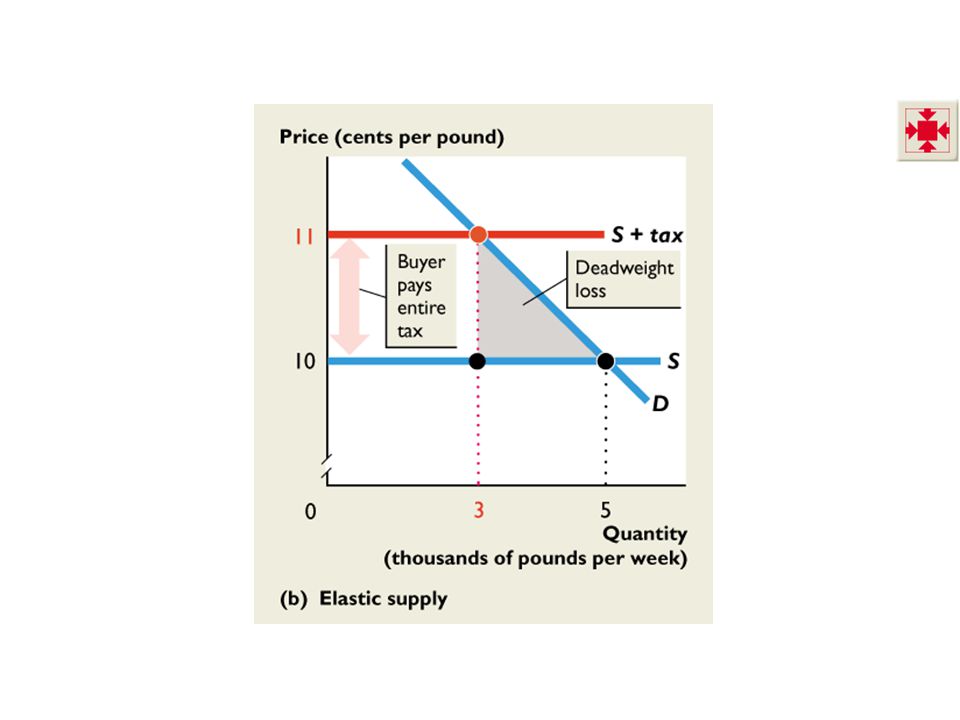
Figure 7.4(b) shows tax incidence in a market with perfectly elastic supply—the market for sand.
A tax of 1¢ a pound increases the price by 1¢ a pound, and the buyer pays all the tax.
A deadweight loss arises, so the outcome is inefficient.

30. 7.2 PRICE CEILINGS
A price ceiling or price cap is a government regulation that places an upper limit on the price at which a particular good, service, or factor of production may be traded.
An example is a price ceiling on housing rents.
Trading above the price ceiling is illegal.

31. A Rent Ceiling (Rent control)
7.2 PRICE CEILINGS
A Rent Ceiling (Rent control)
A rent ceiling is a regulation that makes it illegal to charge more than a specified rent for housing.
The effect of a rent ceiling depends on whether it is imposed at a level above or below the market equilibrium rent.
Ask the students if they saw the article in the day’s local paper that the local government plans to place a $200 limit on rents that landlords could charge for apartments near campus. (Of course this story wasn’t in the paper, but students are more likely to pay attention if they think you’re serious! Don’t tell them this yet though.) Ask them to participate in an informal vote by raising a hand in response to “Who thinks this is a good idea?”, “Who thinks this is a bad idea?”, and “Who doesn’t care?” (This last one always catches a few honest students who like to chuckle as they raise their hands!)
Then explain to the students that this limit is called a “rent ceiling” and cities across the country have them…so they must be good, right? However, further explain that in this lecture, they’ll find out several ways that the government intervenes in markets and that while the ideas might sound good, economically they create problems. At the end of the lecture, remark how astute the students were that voted against the price ceilings and definitely be sure to tell the students that the local government isn’t really going to impose the rent ceiling.

32. 7.2 PRICE CEILINGS Figure 7.5 shows a housing market.
1. At the market equilibrium
2. The equilibrium rent is $550 a month and
3. The equilibrium quantity is 4,000 units of housing.
If a rent ceiling is set above $550 a month, nothing will change.

33. The “Eye on the Past” in the chapter has a fascinating story of the 1906 earthquake in San Francisco. This story is well worth telling, not only for itself but also because it allows you to correct a mistake that a vast number of students make. In particular, many students think that an earthquake that destroys housing increases the demand for housing. I find the easiest way to explain that the earthquake has no effect on the demand is to use some simple numbers. Assume that before the earthquake, at the equilibrium rent there are 100 people demanding 100 apartments. Point out to your students that at this rent the quantity of apartments demanded is 100 and that all 100 people demanding an apartment have one. Now, suppose an earthquake (or other natural disaster) strikes so that at the initial rent the quantity of apartments supplied is only 60. So, of the 100 people demanding apartments, now 60 have apartments and 40 are homeless. The point is that there are still 100 people demanding apartments (only now 60 have apartments while 40 are still looking), so the quantity demanded has not changed. It is the supply that has changed, not the demand. Moreover, the fact there is a shortage of 40 apartments, so that 40 people are still searching for an apartment, is what leads to an increase in the equilibrium rent.
Use the separate PPT slide show on this “Eye On”.

34. 7.2 PRICE CEILINGS
Figure 7.6 shows how a rent ceiling creates a shortage.
A rent ceiling is imposed at $400 a month, which is below the market equilibrium rent.
1. The quantity of housing supplied decreases to 3,000 units.
When you use a demand-supply graph to show the effects of a price ceiling or price floor, be sure to label all the prices, quantities, and the ceiling or floor. In the case of the price ceiling, clearly label and emphasize the shortage created. In the case of the price floor, clearly label and emphasize the surplus created. As you add more lines to the demand-supply graph, there is always the chance for confusion. Many times the students leave the labels off, and when they go back to study, they can’t remember what that extra line is. So, be sure that you label the lines and stress to your class that they should be doing the same. Use price ceilings and floors to remind students that any surplus or shortage is a horizontal distance. Some students want to look at vertical distances or areas of triangles as the measure of the surplus or shortage.
2. The quantity of housing demanded increases to 6,000 units.
3. A shortage of 3,000 units arises.

35. Emphasize that the shaded illegal region is out of bounds.

36. 7.2 PRICE CEILINGS
When a rent ceiling creates a housing shortage, two developments occur:
A black market
Increased search activity
A black market is an illegal market that operates alongside a government-regulated market.
Search activity is the time spent looking for someone with whom to do business.

37. 7.2 PRICE CEILINGS
Figure 7.7 shows how a rent ceiling creates a black market and housing search.
With a rent ceiling of $400 a month:
1. 3,000 units of housing are available.
2. Someone is willing to pay $625 a month for the 3,000th unit of housing.

38. 7.2 PRICE CEILINGS
3. Black market rents might be as high as $625 a month and resources get used up in costly search activity.

40. Are Rent Ceilings Efficient?
7.2 PRICE CEILINGS
Are Rent Ceilings Efficient?
With a rent ceiling, the outcome is inefficient.
Marginal benefit exceeds marginal cost.
Total surplus—the sum of producer surplus and consumer surplus—shrinks and a deadweight loss arises.
People who can’t find housing and landlords who can’t offer housing at a lower rent lose.

41. 7.2 PRICE CEILINGS Figure 7.8(a) shows an efficient housing market.
1. The market is efficient with marginal benefit equal to marginal cost.
2. Consumer surplus plus
3. Producer surplus is as large as possible.

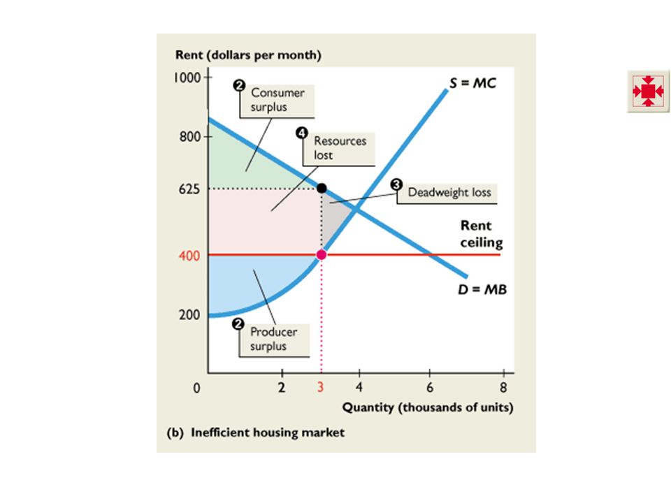
43. 7.2 PRICE CEILINGS
Figure 7.8(b) shows the inefficiency of a rent ceiling.
A rent ceiling restricts the quantity supplied and marginal benefit exceeds marginal cost.
1. Consumer surplus shrinks.
2. Producer surplus shrinks.

44. 7.2 PRICE CEILINGS 3. A deadweight loss arises.
4. Other resources are lost in search activity and evading and enforcing the rent ceiling law .
Resource use is inefficient.

46. Are Rent Ceilings Fair? 7.2 PRICE CEILINGS Are the rules fair?
Are the results fair?
Does blocking rent adjustments avoid scarcity?
What mechanisms allocate resources when prices don’t do the job?
Are those non-price mechanisms fair?

47. If Rent Ceilings Are So Bad, Why Do We Have Them?
7.2 PRICE CEILINGS
If Rent Ceilings Are So Bad, Why Do We Have Them?
Current renters gain and lobby politicians.
More renters than landlords, so rent ceilings can tip an election.

48. 7.3 PRICE FLOORS
A price floor is a government regulation that places a lower limit on the price at which a particular good, service, or factor of production may be traded.
An example is the minimum wage in labor markets.
Trading below the price floor is illegal.

49. 7.3 PRICE FLOORS Figure 7.9 shows a market for fast-food servers.
1. The demand for and supply of fast-food servers determine the market equilibrium
2. The equilibrium wage rate is $5 an hour.
3. The equilibrium quantity is 5,000 servers.

51. 7.3 PRICE FLOORS
The Minimum Wage
A minimum wage law is a government regulation that makes hiring labor for less than a specified wage illegal.
Firms can pay a wage rate above the minimum wage but they may not pay a wage rate below the minimum wage.
The effect of a minimum wage depends on whether it is set above or below the market equilibrium wage rate.
To launch your lecture on the minimum wage, ask the students about jobs around town. Sound them out to see if there are a lot of jobs that pay the minimum wage. (Do not ask a particular student his or her wage, because he or she may be embarrassed if the wage is the minimum wage!) Then, ask the students if they think jobs would be easier or harder to find without the minimum wage. You can easily segue from the students’ answers to your lecture on the minimum wage and you also can easily interweave their answers into your lecture.

52. 7.3 PRICE FLOORS
Figure 7.10 shows how a minimum wage creates unemployment.
A minimum wage is set at $7 an hour, above the equilibrium wage.
1. The quantity of labor demanded decreases to 3,000 workers.
Again, emphasize that the shaded illegal region is out of bounds.
2. The quantity of labor supplied increases to 7,000 people.
3. 4,000 people are unemployed.

54. Is the Minimum Wage Efficient?
7.3 PRICE FLOORS
Is the Minimum Wage Efficient?
The firms’ surplus and workers’ surplus shrink, and a deadweight loss arises.
Firms that cut back employment and people who can’t find jobs at the higher wage rate lose.
The total loss exceeds the deadweight loss because resources get used in costly job-search activity.

55. 7.3 PRICE FLOORS Figure 7.12(a) shows an efficient labor market.
1. At the market equilibrium, the marginal benefit of labor to firms equals the marginal cost of working.
2. The sum of the firms’ and workers’ surpluses is as large as possible.

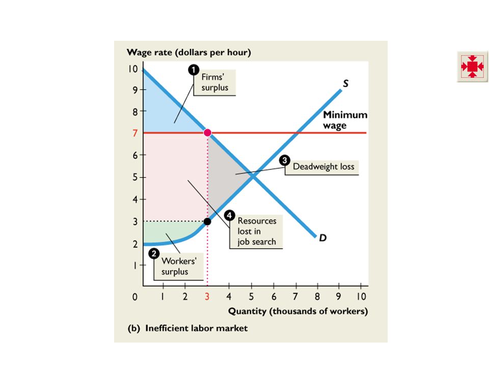
57. 7.3 PRICE FLOORS
Figure 7.12(b) shows an inefficient labor market with a minimum wage.
The minimum wage restricts the quantity demanded.
1. The firms’ surplus shrinks.
2. The workers’ surplus shrinks.

58. 7.3 PRICE FLOORS 3. A deadweight loss arises.
4. Other resources are used up in job-search activity.
The outcome is inefficient.

60. Is the Minimum Wage Fair?
7.3 PRICE FLOORS
Is the Minimum Wage Fair?
Is the rule fair?
Is the result fair?
If the wage rate doesn’t allocate labor, what does?
Are non-wage allocation mechanisms fair?

61. If the Minimum Wage Is So Bad, Why Do We Have It?
7.3 PRICE FLOORS
If the Minimum Wage Is So Bad, Why Do We Have It?
The effects of minimum wage on employment might be small, and the effects on poverty rates are smaller.
What would make the effects on employment small?
Why would effect on poverty rates be small?