Conventional Data Mining Techniques II

Conventional Data Mining Techniques II
Computers are useless. They can only give you answers. –Pablo Picasso A B M Shawkat Ali Pablo Picasso PowerPoint permissions Cengage Learning Australia hereby permits the usage and posting of our copyright controlled PowerPoint slide content for all courses wherein the associated text has been adopted. PowerPoint slides may be placed on course management systems that operate under a controlled environment (accessed restricted to enrolled students, instructors and content administrators). Cengage Learning Australia does not require a copyright clearance form for the usage of PowerPoint slides as outlined above. Copyright © 2007 Cengage Learning Australia Pty Limited

My Request “A good listener is not only popular everywhere, but after a while he gets to know something” - Wilson Mizner Computers are useless. They can only give you answers. –Pablo Picasso; The world is governed more by appearances rather than realities… --Daniel Webster; Life is pleasant. Death is peaceful. It’s the transition that’s troublesome. –Isaac Asimov

Association Rule Mining
PowerPoint permissions Cengage Learning Australia hereby permits the usage and posting of our copyright controlled PowerPoint slide content for all courses wherein the associated text has been adopted. PowerPoint slides may be placed on course management systems that operate under a controlled environment (accessed restricted to enrolled students, instructors and content administrators). Cengage Learning Australia does not require a copyright clearance form for the usage of PowerPoint slides as outlined above. Copyright © 2007 Cengage Learning Australia Pty Limited

Objectives On completion of this lecture you should know:
Features of association rule mining. Apriori: Most popular association rule mining algorithm. Association rules evaluation. Association rule mining using WEKA. Strengths and weaknesses of association rule mining. Applications of association rule mining.

Association rules Affinity Analysis
Market Basket Analysis: Which products go together in a basket? Uses: determine marketing strategy, plan promotions, shelf layout. Looks like production rules, but more than one attribute may appear in the consequent. IF customers purchase milk THEN they purchase bread AND sugar

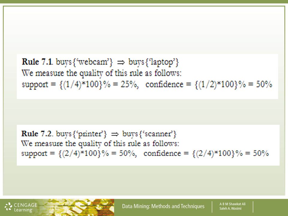
Transaction data Table 7.1. Transactions Data Transaction ID
Itemset or Basket 01 {‘webcam’, ‘laptop’, ‘printer’} 02 {‘laptop’, ‘printer’, ‘scanner’} 03 {‘desktop’, ‘printer’, ‘scanner’} 04 {‘desktop’, ‘printer’, ‘webcam’}

Concepts of association rules
Rule for Support: The minimum percentage of instances in the database that contain all items listed in a given association rule.

Example 5,000 transactions contain milk and bread in a set of 50,000
Support => 5,000 / 50,000 = 10%

Concepts of association rules
Rule for Confidence: Given a rule of the form “If A then B”, rule for confidence is the conditional probability that B is true when A is known to be true.

Example IF customers purchase milk THEN they also purchase bread:
In a set of 50,000, there are 10,000 transactions that contain milk, and 5,000 of these contain also bread. Confidence => 5,000 / 10,000= 50%

Parameters of ARM To find all items that appears frequently in
transactions. The level of frequency of appearance is determined by pre-specified minimum support count. Any item or set of items that occur less frequently than this minimum support level are not included for analysis.

2. To find strong associations among the frequent items.
The strength of the association is quantified by the confidence. Any association below a pre-specified level of confidence is not used to generate rules.

Relevance of ARM On Thursdays, grocery store consumers often purchase diapers and beer together. Customers who buy a new car are very likely to purchase vehicle extended warranty. When a new hardware store opens, one of the most commonly sold items is toilet fittings.

Functions of ARM Finding the set of items that has significant impact on the business. Collating information from numerous transactions on these items from many disparate sources. Generating rules on significant items from counts in transactions.

Single-dimensional association rules
Table 7.2 Boolean form of a transaction data. Transaction id ‘webcam’ ‘laptop’ ‘printer’ ‘scanner’ ‘desktop’ 01 1 02 03 04 (cont.)

Multidimensional association rules

General considerations
We are interested in association rules that show a lift in product sales where the lift is the result of the product’s association with one or more other products. We are also interested in association rules that show a lower than expected confidence for a particular association.

{‘printer’, ‘scanner’} {‘printer’, ‘desktop’} {‘scanner’, ‘desktop’}
Itemset Supports in % ‘Webcam’ 50% ‘Laptop’ ‘Printer’ 100% ‘Scanner’ ‘Desktop’ { ‘webcam’, ‘laptop’} 25% {‘webcam’, ‘printer’ } {‘webcam’, ‘scanner’} 00% {‘webcam’, ‘desktop’} {‘laptop’, ‘printer’} {‘laptop’, ‘scanner’} {‘laptop’, ‘desktop’} {‘printer’, ‘scanner’} {‘printer’, ‘desktop’} {‘scanner’, ‘desktop’} {‘webcam’, ‘laptop’, ‘printer’} {‘webcam’, ‘laptop’, ‘scanner’} {‘webcam’, ‘laptop’, ‘desktop’} {‘laptop’, ‘printer’, ‘scanner’} {‘laptop’, ‘printer’, ‘desktop’} {‘printer’, ‘scanner’, ‘desktop’} {‘webcam’, ‘laptop’, ‘printer’, ‘scanner’, desktop’} Table 7.3 Support measure for the items/sets of items in transactional data.

Enumeration tree Figure 7.1 Enumeration tree of transaction items of Table 7.1. In the left nodes, branches reduce by 1 for each downward progression – starting with 5 branches and ending with 1 branch, which is typical

Association models nCk = The number of combinations of n things taken k at a time.

Two other parameters Improvement (IMP) = Share (SH) =
where LMV = local measure value and TMV is total measure value.

IMP and SH measure (cont.) Table 7.4. Market transaction data
Transaction ID ‘Yogurt’ (A) ‘Cheese’ (B) ‘Rice’ (C) ‘Corn’ (D) T1 2 5 10 T2 3 T3 20 T4 12 T5 13 (cont.)

Table 7.5 Share measurement
‘Yogurt’(A) ‘Cheese’(B) ‘Rice’(C) ‘Corn’(D) Itemset LMV SH A 10 0.10 B 15 0.15 C 35 0.35 D 40 0.40 AB 8 0.08 12 0.12 20 0.20 AC 7 0.07 25 0.25 32 0.32 AD 5 0.05 22 0.22 27 0.27 BC 2 0.02 BD 13 0.13 17 0.17 30 0.30 CD 23 0.23 38 0.38 ABC ABD 3 0.03 ACD BCD 0.00 ABCD

Taxonomies Low-support products are lumped into bigger categories and high-support products are broken up into subgroups. Examples are: Different kinds of potato chips can be lumped with other munchies into snacks, and ice cream can be broken down into different flavours.

Large Datasets The number of combinations that can generate from transactions in an ordinary supermarket can be in the billions and trillions. The amount of computation thus required for Association Rule Mining can stretch any computer.

APRIORI algorithm All singleton itemsets are candidates in the first pass. Any item that has a support value of less than a specified minimum is eliminated. 2. Selected singleton itemsets are combined to form two-member candidate itemsets. Again, only the candidates above the pre-specified support value are retained. (cont.)

3. The next pass creates three-member candidate itemsets and the process is repeated. The process stops only when all large itemsets are accounted for. 4. Association Rules for the largest itemsets are created first and then rules for the subsets are created recursively.

Figure 7.2 Graphical demonstration of the working of the Apriori algorithm

APRIORI in Weka Step 1. Let us open the ‘market-basket.arff’ data file from the book toolkit CD and we will get the window as shown in Figure 7.3. Figure 7.3 Weka environment with market-basket.arff data file

Step 2 Figure 7.4 Spend98 attribute information visualisation.
Step 2. Next, we delete attribute 13 since we wish to focus on response to one promotion only. This can be accomplished by clicking on this attribute, which will result in a tick sign on the empty box to its left, and then clicking on remove. After this task the Weka window will display as shown in Figure 7.4. Figure 7.4 Spend98 attribute information visualisation.

Step 3 Figure 7.5 Target attributes selection through Weka
Step 3. We know that an ARM algorithm cannot handle numeric attributes. Therefore, discretization of all numeric data has to be done. This can be accomplished through Weka’s internal discretization tools. Let us first click on ALL under the Attributes window which will result in tick signs appearing in all empty boxes preceding the attributes. Since the last two attributes are not numeric, so we have to remove the tick signs from these two attributes. The resulting Weka window will display as show in Figure 7.5. Figure 7.5 Target attributes selection through Weka

Step 4 Figure 7.6 Discretisation filter selection
Step 4. The Weka discretisation filter, can divide the ranges blindly, or use various statistical techniques to automatically determine the best way of partitioning the data. In this case, we will perform simple binning. To change the defaults for this filter, we have to click on the Choose button. This will open the Discretise Filter dialogue box. Next, we have to follow the link: Weka filters unsupervised attribute Discretise as shown in Figure 7.6. Figure 7.6 Discretisation filter selection

Step 5 Figure 7.7 Parameter selections for discretisation.
Step 5. We divide each numeric attribute into 3 bins (intervals). We choose the number of bins by clicking on Discretise when the new window displayed in Figure 7.7 would appear. In the dialogue box we select False to all other options. Figure 7.7 Parameter selections for discretisation.

Step 6 Figure 7.8 Descretisation activation
Step 6. To execute filtering, we have to click on Apply in the Filter panel. This will result in changes in right panel for Selected attribute as shown in Figure 7.8. Both Figures 7.5 and 7.8 display the information about the attribute ‘Grocery.’ If we compare the two figures, we can clearly notice the difference. In Figure 7.8, the attribute has been separated into 3 bins {'(-inf )', '( )' and '( inf)'} and the frequency of each bin is {778, 198 and 24}. Figure 7.8 Descretisation activation

Discretised data visualisation
Figure 7.9 Discretised data visualisation

Step 7 Figure 7.10 Apriori algorithm selection from Weka for ARM
Step 7. To start ARM now, we should click on the Associate tab in the Weka main menu which will bring up the interface for the association rule algorithms. Apriori algorithm is the default selection and we will get the window as displayed in Figure If we decide to change any of the default parameter setting we can do that by clicking on “Apriori”, which will bring up a dialogue box, and then making our selection in the dialogue box. Figure Apriori algorithm selection from Weka for ARM

Step 8 Figure 7.11 Apriori output
Step 8. To start execution of the algorithm, we should click on the Start button and the window will display all the characteristics of the execution process. After completion we will get the Apriori outcome in the Weka window as displayed in Figure 7.11. Figure Apriori output

Associator output ‘Dairy’='(-inf ]’ ‘Deli’='(-inf ]' 847 ==> ‘Bakery’='(-inf ]‘ conf:(0.98)

Strengths and weaknesses
Easy Interpretation Easy Start Flexible Data Formats Simplicity Exponential Growth in Computations Lumping Rule Selection

Applications of ARM Store Layout Changes Cross/Up selling
Disaster Weather forecasting Remote Sensing Gene Expression Profiling

Recap What is association rule mining?
Apriori: Most popular association rule mining algorithm. Applications of association rule mining.

The Clustering Task PowerPoint permissions Cengage Learning Australia hereby permits the usage and posting of our copyright controlled PowerPoint slide content for all courses wherein the associated text has been adopted. PowerPoint slides may be placed on course management systems that operate under a controlled environment (accessed restricted to enrolled students, instructors and content administrators). Cengage Learning Australia does not require a copyright clearance form for the usage of PowerPoint slides as outlined above. Copyright © 2007 Cengage Learning Australia Pty Limited

Unsupervised clustering technique Measures for clustering performance Clustering algorithms Clustering task demonstration using WEKA Applications, strengths and weaknesses of the algorithms

Clustering: Unsupervised learning
Clustering is a very common technique that appears in many different settings (not necessarily in a data mining context) Grouping “similar products” together to improve the efficiency of a production line Packing “similar items” into a basket Grouping “similar customers” together Grouping “similar stocks” together

A simple clustering example
Table 8.1 A simple unsupervised problem Sl. No. Subjects Code Marks 1 COIT21002 85 2 COIS11021 78 3 COIS32111 75 4 COIT43210 83

Cluster representation
Figure 8.1 Basic clustering for data of Table 8.1.The X-axis is the serial number and Y-axis is the marks

How many clusters can you form?
A A A A K K K K Q Q Q Q J J J J Figure 8.2 Simple playing card data

Distance measure The similarity is usually captured by a distance measure. The original proposed measure of distance is the Euclidean distance.

Figure 8.3 Euclidean distance D between two points A and B

Other distance measures
City-block (Manhattan) distance Chebychev distance: Maximum Power distance: Minkowski distance when p = r.

Distance measure for categorical data
Percent disagreement

Types of clustering Hierarchical Clustering Agglomerative Divisive

Agglomerative clustering
Place each instance into a separate partition. Until all instances are part of a single cluster: a. Determine the two most similar clusters. b. Merge the clusters chosen into a single cluster. 3. Choose a clustering formed by one of the step 2 iterations as a final result.

Dendrogram

Example 8.1 Figure 8.5 Hypothetical data points for agglomerative clustering

Example 8.1 cont. Step 1 Step 2 Step 3
C = {{P1}, {P2}, {P3}, {P4}, {P5}, {P6}, {P7}, {P8}} Step 2 Step 3

Example 8.1 cont. Step 4 Step 5 Step 6 Step 7

Agglomerative clustering: An example
Figure 8.6 Hierarchical clustering of the data points of Example 8.1

Dendrogram of the example
Figure 8.7 The dendrogram of the data points of Example 8.1

Types of clustering cont.
Non-Hierarchical Clustering Partitioning methods Density-based methods Probability-based methods

Partitioning methods The K-Means Algorithm:
Choose a value for K, the total number of clusters. Randomly choose K points as cluster centers. Assign the remaining instances to their closest cluster center. Calculate a new cluster center for each cluster. Repeat steps 3-5 until the cluster centers do not change.

General considerations of K-means algorithm
Requires real-valued data. We must pre-select the number of clusters present in the data. Works best when the clusters in the data are of approximately equal size. Attribute significance cannot be determined. Lacks explanation capabilities.

Example 8.2 Let us consider the dataset of Example 8.1 to find two clusters using the k-means algorithm. Step 1. Arbitrarily, let us choose two cluster centers to be the data points P5 (5, 2) and P7 (1, 2). Their relative positions can be seen in Figure 8.6. We could have started with any two other points. The initial selection of points does not affect the final result.

Step 2. Let us find the Euclidean distances of all the data points from these two cluster centers.

Step 2. (Cont.)

Step 3. The new cluster centres are:

Step 4. The distances of all data points from these new cluster centres are:

Step 4. (cont.)

Step 5. By the closest centre criteria P5 should be moved from C2 to C1, and the new clusters are C1 = {P1, P5, P6, P7, P8} and C2 = {P2, P3, P4}. The new cluster centres are:

Step 6. We may repeat the computations of Step 4 and we will find that no data point will switch clusters. Therefore, the iteration stops and the final clusters are C1 = {P1, P5, P6, P7, P8} and C2 = {P2, P3, P4}.

Density-based methods
Figure 8.8 (a) Three irregular shaped clusters (b) Influence curve of a point

Probability-based methods
Expectation Maximization (EM) uses a Gaussian mixture model: Guess initial values of all the parameters until a termination criterion is achieved Use the probability density function to compute the cluster probability for each instance. Use the probability score assigned to each instance in the above step to re-estimate the parameters.

Clustering through Weka
Step 1. Step 1. Let us open the ‘credit-g.arff’ data file from the Weka data directory using WEKA Explorer interface and we will get a screen display as shown in Figure 8.9. Figure 8.9 Weka environment with credit-g.arff data

Step 2. Figure 8.10 SimpleKMeans algorithm and its parameter selection
Step 2. To perform the clustering task we have to click on the Cluster tab in the Weka Explorer and click on the Choose button. We will see a list of available clustering algorithms in the drop down list. In our case, we select SimpleKMeans. Next, by clicking on the text box to the right of the Choose button, we get the pop-up window as shown in Figure There are two parameters we can select from that window: one is the number of clusters we are seeking, and the other is the number for the seed clusters. Figure SimpleKMeans algorithm and its parameter selection

Step 3. Figure 8.11 K-means clustering performance
Step 3. Once the parameters have been specified, we can run the clustering algorithm. Here we make sure that in the Cluster Mode panel, the Use training set option is selected, and we click Start. After the bird stops moving and sits, we will see the Weka window as shown in Figure 8.11. Figure K-means clustering performance

Step 3. (cont.) Figure Weka result window

Cluster visualisation
Figure Cluster visualisation

Individual cluster information
Figure Cluster0 instances information

Step 4. Figure 8.15 Cluster 1 instance information
Step 4. We can change the parameter values and even algorithms still dwelling on the same problem, and watch for better clustering performance. When we stop the clustering process with results that appear satisfactory, we have to seek expertise to specify appropriate names that meaningfully refers to different clusters. Figure Cluster 1 instance information

Kohonen neural network
Figure A Kohonen network with two input nodes and nine output nodes

Kohonen self-organising maps:
Contains only an input layer and an output layer but no hidden layer. The number of nodes in the output layer that finally captures all the instances determine the number of clusters in the data.

Example 8.3 In this example we illustrate how the nodes in the output layer are rewarded and what procedure is followed to change the connection weights in the network. For simplicity, we use two input nodes and two output nodes only. This network is shown in Figure We consider only one instance whose input into node Input 1 is 0.3 and into node Input 2 is 0.6. The initial connection weights are also shown in the figure. Figure 8.17 Connections between input and output nodes of a neural network

Example 8.3 Cont. The scoring for any output node k is done using the formula: = 0.447 = 0.141

Example 8.3 cont.

Example 8.3 cont. Assuming that the learning rate is 0.3, we get:

Cluster validation t-test -test Validity in Test Cases

Unsupervised Learning Diverse Data Types Easy to Apply Similarity Measures Model Parameters Interpretation

Applications of clustering algorithms
Biology Marketing research Library Science City Planning Disaster Studies Worldwide Web Social Network Analysis Image Segmentation

Recap What is clustering? K-means: Most popular clustering algorithm
Applications of clustering techniques

The Estimation Task PowerPoint permissions Cengage Learning Australia hereby permits the usage and posting of our copyright controlled PowerPoint slide content for all courses wherein the associated text has been adopted. PowerPoint slides may be placed on course management systems that operate under a controlled environment (accessed restricted to enrolled students, instructors and content administrators). Cengage Learning Australia does not require a copyright clearance form for the usage of PowerPoint slides as outlined above. Copyright © 2007 Cengage Learning Australia Pty Limited

Assess the numeric value of a variable from other related variables. Predict the behaviour of one variable from the behaviour of related variables. Discuss the reliability of different methods of estimation and perform a comparative study.

What is estimation? Finding the numeric value of an unknown attribute from observations made on other related attributes. The unknown attribute is called the dependent (or response or output) attribute (or variable) and the known related attributes are called the independent (or explanatory or input) attributes (or variables).

Scatter Plots and Correlation
Week ending ASX BHP RIO 33.70 23.35 68.80 34.95 23.73 70.50 34.14 24.66 74.00 34.72 26.05 76.10 34.61 25.53 74.75 34.28 24.75 74.40 33.24 23.88 71.65 33.14 24.55 72.20 31.08 24.34 70.35 31.72 23.37 67.50 33.30 24.70 71.25 32.60 25.92 75.23 32.70 28.00 78.85 33.20 29.50 83.70 29.75 82.32 32.50 30.68 83.06 Table 9.1 Weekly closing stock prices (in dollars) at the Australian Stock Exchange

Figure 9.1a Computer screen-shots of Microsoft Excel spreadsheets to
demonstrate plotting of scatter plot

Figure 9.1b

Figure 9.1c

Figure 9.1d

Figure 9.1e Computer screen-shots of Microsoft Excel spreadsheets to
demonstrate plotting of scatter plot

Correlation coefficient

Scatter plots of X and Y variables and their correlation coefficients
Figure 9.2 Scatter plots of X and Y variables and their correlation coefficients

CORREL xls function Figure 9.3 Microsoft Excel command for the correlation coefficient

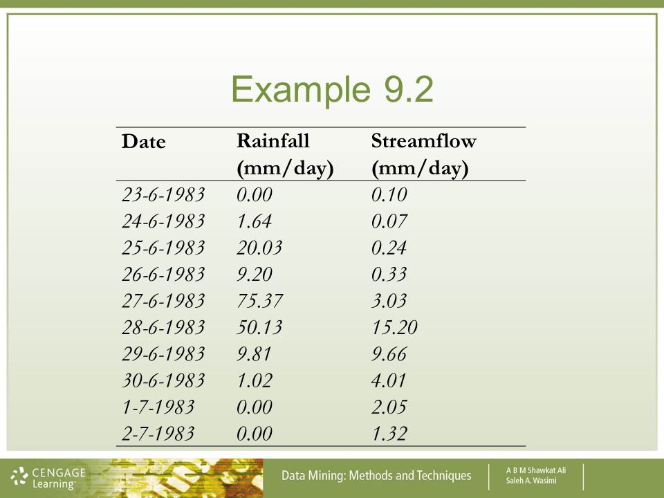
Example 9.2 Date Rainfall (mm/day) Streamflow (mm/day) 23-6-1983 0.00
0.10 1.64 0.07 20.03 0.24 9.20 0.33 75.37 3.03 50.13 15.20 9.81 9.66 1.02 4.01 2.05 1.32

Example 9.2 cont. The computations can be done neatly in tabular form as given in the next slide: (a) For the mean values: = /10 = 16.72, = /10 = 3.601

Example 9.2 cont. Therefore, the correlation coefficient, r =

Linear regression analysis
Linear means all exponents (powers) of x must be one, i.e., it cannot be a fraction or a value greater than 1. There cannot be a product term of variables as well.

Fitting a straight line
y = m x + c Suppose the line passes through two points A and B, where A is (x1,y1) and B is (x2, y2). Eq. 9.3 where y is the value of the dependent variable for the x value of the independent variable, m is the slope and c is the intercept.

Example 9.3 Problem: The number of public servants claiming compensation for stress has been steadily rising in Australia. The number of successful claims in was 800 while in the figure was How many claims are expected in the year if the growth continues steadily? If each claim costs an average of $24,000, what should be the budget allocation of Comcare in year for stress-related compensation?

Example 9.3 cont. Therefore, using equation (9.3) we get:
Solving, we have Y = 220.X – 437,000. If we now let X = 2007, we get the expected number of claims in the year So the number of claims in the year is expected to be 220(2007) – 437,000 = 4,540. At $24,000 per claim, Comcare's budget should be $108,960,000.

Simple linear regression
Figure 9.6 Schematic representation of the simple linear regression model

Least squares criteria

Example 9.5 Table 9.2 Unisuper membership by States State No. of
Inst., X Membership, Y X2 Y2 XY NSW 17 5 987 289 x107 QLD 11 5 950 121 x107 65 450 SA 10 3 588 100 x107 35 880 TAS 3 1 356 9 x106 4 068 VIC 41 14 127 1681 x108 WA 4 847 81 x107 43 623 Others 3 893 x107 42 823 Total 102 39 748 2402 x108

Example 9.5 cont. b1 = Sxy/Sxx = /915.7 = 320.7 = (320.7)(14.57) = 1005 Therefore, the regression equation is Y = 320.7X

Multiple linear regression with Excel
Type regression under help and then go to linest function. Highlight ‘District office building data’ and copy with cntrl C and paste with cntrl V in your spreadsheet.

Multiple regression Where Y is the dependent variable; X1, X2, ... are independent variables; 0,1, ... are regression coefficients; and a,b,... are exponents.

Example 9.6 Period No. of Private Houses Average weekly earnings ($)
No. of persons in workforce (in millions) Variable Home loan rate (in %) 83 973 428 5.6889 15.50 454 5.8227 13.50 487 6.0333 17.00 96 390 521 6.1922 16.50 87 038 555 6.0933 13.00 581 5.8846 10.50 591 5.8372 9.50 609 5.9293 8.75 634 6.1190 = LINEST (A2:A10,B2:D10,TRUE,TRUE)

Example 9.6 cont. Hence, from the printout, the regression equation is
The Ctrl and Shift keys must be kept depressed while striking the Enter key to get tabular output. Figure 9.7 Demonstration of use of LINEST function Hence, from the printout, the regression equation is the following:H =  E –  W I

Coefficient of determination
If the fit is perfect, the R2 value will be one and if there is no relationship at all, the R2 value will be zero.

Logistic regression Regression equation cannot model discrete values. We get a better reflection of the reality if we replace the actual values by its probability. The ratio of the probabilities of occurrence and non-occurrence directs us close to the actual value.

Transforming the linear regression model
Logistic regression is a nonlinear regression technique that associates a conditional probability with each data instance.

The logistic regression model
. ax in the right-hand side of the regression equation in vector form.

Logistic regression cont.
Figure 9.8 Graphical representation of the logistic regression equation

Regression in Weka Figure Selection of logistic function

Output from logistic regression
Figure Output from logistic regression

Visualisation option of the results
Figure Visualisation option of the results

Visual impression of data and clusters
Figure Visual impression of data and clusters

Particular instance information
Figure 9.15 Information about a particular instance

Regression analysis is a powerful tool suitable for linear relationships, but most real-world problems are nonlinear. Mostly, therefore, the output is not accurate but useful. Regression techniques assume normality in the distribution of uncertainty and the instances are assumed to be independent of each other. This is not the case with many real problems.

Applications of regression algorithms
Financial Markets Medical Science Retail Industry Environment Social Science

Recap What is estimation? How to solve the estimation problem?
Applications of regression analysis.

Conventional Data Mining Techniques II

Similar presentations

Presentation on theme: "Conventional Data Mining Techniques II"— Presentation transcript:

Similar presentations

About project

Feedback

Log in

Auth with social network:

Conventional Data Mining Techniques II

Similar presentations

Presentation on theme: "Conventional Data Mining Techniques II"— Presentation transcript:

Similar presentations

About project

Feedback