1. Control System Analysis and Design by the Frequency Response Method
Chapter 7
Control System Analysis and Design by the Frequency Response Method

2. 7-1 Introduction
1. The concept of frequency response
G(s)
R(s)
Y(s)

3. Frequency response:
The frequency response of a system is defined as the steady-state response of the system to a sinusoidal input signal.
For a stable LTI system, the resulting output signal, as well as signals throughout the system, is also sinusoidal in the steady-state; it differs from the input waveform only in amplitude and phase angle.

4. 2. Obtaining steady-state outputs to sinusoidal inputs
For a given stable LTI system with a sinusoidal input, the steady state output can be completely characterized by its transfer function with s being replaced by j. That is, if the system transfer function is G(s), then from the steady-state response
we have

5. To prove this conclusion, consider the following controlled plant:
G(s)
R(s)
Y(s)

6. G(s)
R(s)
Y(s)
Transient response
Steady-state response
If the system is stable, then the transient response

7. The steady state response
Note that
Hence,

8. Write
where
Similarly,
Therefore,

9. Now, the steady-state response can be written as
with
and

10. based on which, we obtain the following important results:
Amplitude ratio of the output
sinusoid to the input sinusoid
Phase shift of the output sinusoid with respect to the input sinusoid

11. Noting that
It follows that the frequency response characteristics of a stable LTI system to a sinusoidal input can be obtained directly from
which is the complex ratio of output sinusoid to input sinusoid.
Remark: Though we have deduced the frequency response under the assumption that G(s) is stable, it can be extended to the case that G(s) is unstable.

12. Example 1. The controlled plant is
R(s)
Y(s)
Let r(t)=Xsint. Find its frequency response yss(t).
Solution: By definition of frequency response, yss(t) can be completely characterized by G(j), that is,
with

13. Example 2. The controlled plant is
Hence,
where <0.
Example 2. The controlled plant is
R(s)
Y(s)
Let r(t)=Xsint and suppose T1>T2. Find its frequency response yss(t).

14. Solution: By definition,
Since in this example,

15. Since by assumption, T1>T2, it follows that >0.
Definition: A positive phase angle is called phase lead and a negative phase angle is called phase lag.
By this definition, the fist example is a phase lag system, while the second one is a phase lead system.
Therefore, the lead compensator corresponds to a phase lead network while lag compensator, a phase lag network.

16. 3. Why is frequency response important?
Since for an LTI system, its frequency response can be fully characterized by G(j), or by
our later analysis will show that by using the so called Bode diagram and Nyquist plot, one is able to
Determine how the system responds at different frequencies;
Find stability properties of the system in closed-loop control;
Design compensating controllers.

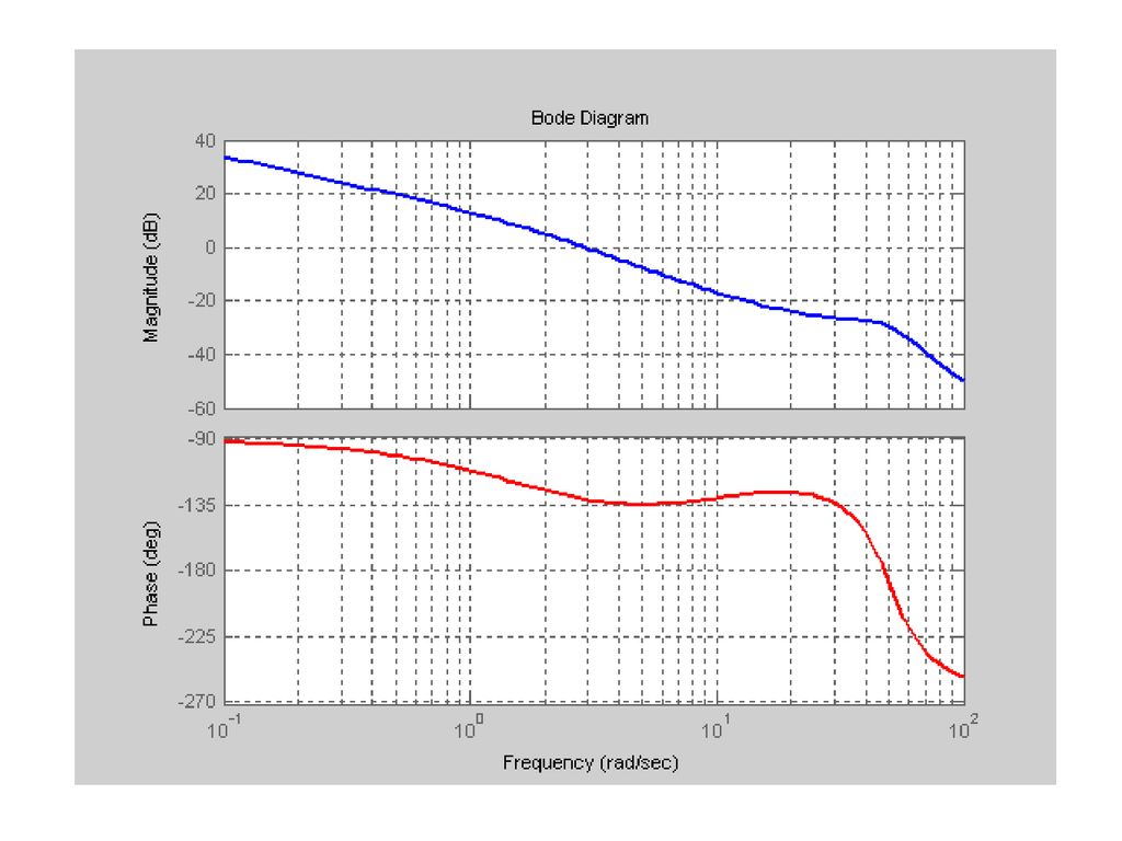
17. 7-2 Bode Diagrams or Logarithmic Plots
Concept of Bode diagram
A Bode diagram consists of two graphs: One is a plot of the logarithm of the magnitude of a sinusoidal transfer function; the other is a plot of phase angle; both are plotted against the frequency on a logarithmic scale. C R

18. where the base of the logarithm is 10, the unit is decibel (dB) and the horizontal axis is logarithmic scale lg.
Bode Phase angle:
with the horizontal axis being also lg.

19. Example. Given a first-order system
Plot its Bode diagram.
Solution: Write
and

20. Hence, both Bode magnitude and phase angle diagrams are shown below:

21. Example. An open-loop transfer function is given below:
Plot its Bode diagram.
Solution: Write
and

22. Bode diagram 10 20 30 40 50 2 4 6 1 8 60

23. From the aforementioned examples, it is clear that one of the main advantages of Bode diagram is that multiplication of magnitude can be converted into addition, which may make our analysis much simpler.

24. 2. Bode diagrams for basic factors of G(j)H(j)
The basic factors that very frequently occur in an arbitrary transfer function G(j)H(j) are

25. 1 10
100
1000
20lgK (dB)  

27. Example. Open-loop transfer functions are
Plot their Bode diagrams.
The bode magnitude plot is the sum of 20lg(10) and -20lg.

28. Bode magnitude:
Phase angle:
Asymptotic curves for Bode magnitude:

29. The frequency 1/T is called corner (break) frequency, at which
Vividly describes the asymptotic curve
The maximum error in the magnitude curve caused by the use of asymptotes occurs at 1/T is approximately equal to 3 dB since

31. First-order derivative factorG(s)=Ts+1:
whose Bode magnitude and phase angle curves, due to the property that Ts+1 is the reciprocal factor of 1/(Ts+1), need only be changed in sign.
Corner frequency: 1/T

32. Example. Open-loop transfer functions are
Plot, for T1>T2 and T1<T2 cases, Bode diagrams.

33. The magnitude of G(j) is
The phase angle of G(j) is

34. From we have 1  r G(j) Resonant frequency: Resonant peak value:Mr
G(j)
Resonant frequency:
When \omega is greater than or equals to 0.707, there is no resonant peak occurs and abs(G(j\omega)) decreases monotonically with maximum value=1=abs(G(j0)).
Resonant peak value:

35. For 0 < 0.707, 1 
0=r
G(j)
and
from which it can be seen that for > 0.707, there is no resonant peak and the magnitude G(j) decreases monotonically as the frequency  increases (20lgG(j)<0 dB, for all values of  > 0. Recall that, for 0.707<< 1, the step response is oscillatory, but the oscillations are well damped and are hardly perceptible).

36. Asymptotic curves for Bode magnitude:
When <<n, the Bode magnitude becomes
When >>n , the Bode magnitude becomes
Therefore, the corner frequency =n.

37. -40dB/dec

38. Note that at n, the phase angle is 900 regardless of  since
If zita is very small the resonant peak cannot be neglectable.

39. Comment on the resonant peak value Mr
For 0 < 0.707,
For  >0.707,

40. Since
it follows that
Zeta=0 corresponds to simple harmonic motion.
This means that if the undamped system is excited at its natural frequency, the magnitude of G(j) becomes infinite.

41. Example. The Bode asymptotic magnitude curve of a second-order system is shown below. Determine its transfer function and resonant peak value.
Solution: The transfer function is of the form: o 30
L()/dB
630
33dB
40dB/dec
Therefore,

42. 3. General procedure for plotting Bode diagrams
1). Write G(s)H(s) in the following normalized form (for instance):
from which the basic factors that compose the transfer function can be obtained.
2). Identify the corner frequencies associated with these basic factors (for instance): 1/1, 1/2, 1/T1, 1/T2, n, and so on.

43. 3). Draw the separate asymptotic magnitude curves for each of the factors:
[-20]
Brown curve

44. Correspondingly, draw the separate phase angle curves for each of the factors:00
450
900

45. 4). Draw the composite curves by algebraically adding the individual curves.

46. Example. The controlled plant is
Draw its asymptotic Bode diagram.
Solution: Note that the system consists of
Constant gain K =10 (20lg10=20 dB)
An integral factor
A first-order factor with corner frequency 2rad/s

47. [-20]
[-40]

48. -20dB/dec
-40dB/dec

49. Example. The controlled plant is
Draw its asymptotic Bode diagram.
A constant gain K=5 (20lgK=14 dB)
An integral factor 1/s
A first-order factor with corner frequency 2rad/s
A first-order derivative factor with corner frequency 10rad/s
A pair of complex poles with corner frequency 50rad/s

51. 40dB

54. Example. The controlled plant is
Draw its asymptotic Bode diagram.
Note that we must rewrite the above transfer function in a normalized form.

55. 4. Minimum phase and nonminimum phase transfer functions
Definition: A transfer function is called a minimum phase transfer function if all its zeros and poles lie in the left-half s-plane, whereas those having poles and zeros in the right-half plane are called nonminimum phase transfer functions.

56. Example. We investigate the range of the phase angles for the following two plants over the entire frequency range from zero to infinity. By definition, G1(s) is a minimum phase transfer function, while G2(s) is a nonminimum phase one.

57. In case of T>T1, G1(s) and G2(s) have same Bode magnitude, but their phase angles are different:
lg
G2(j)
-1800

58. In case of T<T1, G1(s) and G2(s) have same Bode magnitude, but their phase angles are different:

59. In general, we have following conclusion:
For a minimum phase system, the transfer function can be uniquely determined from the magnitude curve alone, while for nonminimum system, this is not the case.
For systems with the same magnitude characteristics, the range in phase angle of the minimum-phase transfer function is minimum among all such systems, while the range in phase angle of any nonminimum-phase transfer function is greater than this minimum.

60. Determine its transfer function and static position error constant Kp.
Example. The Bode magnitude plot of a minimum phase system is shown below: 14 3 10
Determine its transfer function and static position error constant Kp.

61. Solution: The minimum phase assumption implies that the magnitude plot alone suffices to determine its transfer function. The system consists of three factors: gain K, and two first-order factors with corner frequencies 3 rad/s and 10rad/s, respectively. Therefore, the transfer function is
The static position error constant is

62. Determine its transfer function and prove that
Example. The Bode magnitude plot for Type 1 minimum phase system is shown below:
[-20db/dec]
[-40db/dec]
lg
L()
20lgKv
=1 2 3 1
Determine its transfer function and prove that

63. Example. The Bode magnitude plot for type 2 minimum phase system is shown below:
[-40db/dec]
[-20db/dec]
lg
L()
20lgKa
=1
2=
[-60db/dec]
Prove that

64. Example. The asymptotical Bode magnitude plot of a minimum phase system is shown below. Determine its transfer function.
Solution: The minimum phase assumption implies that the transfer function is of the form:

65. The slope of the leftmost curve is 20dB/dec
The slope of the leftmost curve is 20dB/dec. Therefore, the system has an integral factor.
When =1, the y-axis is 15dB, at which the gain is
20lgK=15, K=5.6
When 27, the slope changes from 20dB/dec to 40dB/dec, which shows that =2 is the corner frequency of a first-order system.
=7 is the corner frequency of a first-order derivative factor.
Therefore, the transfer function is

66. 7-3 Polar Plots
1. The concept of Nyquist curve
The Nyquist curve of G(j) is a plot of the magnitude of G(j) versus the phase angle of G(j) on the polar coordinates as  is varied from zero to infinity. Write or

67. Let
Then, as  varies from 0 to +, the terminal of the vector function traces out a curve j 1 O
which is called Nyquist curve, also polar plot.

68. 2. Nyquist plots for basic factors of G(j)H(j)

71. Consider the following network:
Plot its Nyquist curve.

72. A semicircle
Notice: To draw the Nyquist curve, one should choose some typical points, for instance, =0, =1/T and =.

73. Example. Plot the Nyquist curve of the following transfer function:
Since
The low-frequency portion of the curve is

74. The high-frequency portion is
and is tangent to the negative real axis.

75. First-order derivative factor:

76. =0
=
Resonant peak r

77. The low-frequency portion of the curve is
and the high-frequency portion is

78. 3. General shapes of polar plots
We consider the polar plots of general form of transfer function (n>m):
=0, Type 0 systems:
The low-frequency portion of the plot is

79. The high-frequency portion of the plot is
Example. Consider the following transfer function
Sketch its Nyquist plot.

80. Solution:
The low-frequency portion of the plot is
The high-frequency portion of the plot is

81. and is tangent to the negative real axis.
Similarly, we can discuss the Nyquist plot for

82. Example. Consider the following transfer function:
Sketch its Nyquist plot.
If T1, T2> and >T3,

83.  =1, Type 1 systems:
The low frequency portion of the plot is
The high frequency portion of the plot is

84. Example. Consider the following transfer function:
Sketch its Nyquist plots for two cases: <T1, T2 and >T1, T2.
 =2, Type 2 systems:

85. One disadvantage of Nyquist plot is that it does not show clearly the contributions of

86. Example: Let the controlled transfer function be given as
Sketch its Nyquist curve.
Solution: The system consists of four factors: Gain K and two integral factors and a first-order factor. The low-frequency portion of the plot is
and the high-frequency portion of the plot is

87. The sketch of the Nyquist plot is
Example: Let the controlled transfer function be given as
Sketch its Nyquist plots for two cases: <T and >T.

88. Example: Let the controlled transfer function be given as
Sketch its Nyquist curve.

89. Example: Let the controlled transfer function be given as
Sketch its Nyquist curve.

90. Example: Let the controlled transfer function be given as
Sketch its Nyquist curve.
Solution: The system is nonminimum phase. The low-frequency portion of the plot is
and the high-frequency portion of the plot is