1. Measuring & Managing Credit Risk EDF™ Credit Measures for Public Firms
October 2006

2. Session Objectives What is the EDF credit measure?
When does a firm Default?
What drives the EDF credit measure?
How are the EDF Drivers calculated?
How is the EDF measure calculated from the EDF Drivers?
EDF methodology summary
EDF validation
Conclusion 1 2 3 4 5 6 7 8

3. EDF Credit Measure for Public Firms
EDF stands for Expected Default Frequency – the probability that a firm will default within a given time horizon by failing to make an interest or principal payment.
We provide EDF measures for time horizons of 1, 2, 3, 4, and 5 years.
EDF Ranges from .02% to 20%, i.e., 2 to 2000 basis points.
Say we create a portfolio of 100 firms, each with a 2% EDF. On average, 2 out of the 100 firms will default over the next year, and 98 will not default.
A firm with a 2% EDF is 10 times more likely to default than a firm with a 0.2% EDF. 1 2 3 4 5 6 7 8

4. Default Example: Collins & Aikman Corp
Defaulted
May 2005
1-Year EDF
S&P Rating
1-Year EDF
S&P Rating
The value of EDF: Measures credit risk in terms of absolute default probabilities rather than relative rankings.
Provides the most accurate forward-looking, causal model.
Provides frequent updates and early warning of changes in credit quality.
Source: Credit Monitor 1 2 3 4 5 6 7 8

5. Agency Ratings: An Example1 2 3 4 5 6 7 8

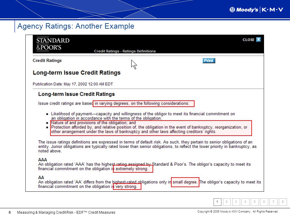
6. Agency Ratings: Another Example1 2 3 4 5 6 7 8

7. Differentiating EDF Credit Measures from Traditional Ratings
Objective, Market driven
Quantitative Method
Quantitative Output
EDF = 0.02% (An actual probability of default)
Absolute (Cardinal)
Precise and continuous, providing full granularity (high resolution)
Specific time horizon
Reflects current assessment of future prospects of the firm/economy
Dynamic, updated daily or monthly
Reflects issuer’s default probability (PD), and not issue-specific LGD
Traditional Ratings
Subjective, driven by fundamental analysis
Qualitative Method
Qualitative Output
AAA = “Obligor’s capacity to meet its financial commitment on the obligation is extremely strong.”
Relative (Ordinal)
Distinct risk buckets without specifying or targeting a specific default rate
No specific time horizon (“long term”)
Supposed to reflect average economic conditions – “through the cycle”
Stable (low ratings volatility)
Opinion on Expected Loss – combines the effect of PD and LGD (Loss Given Default) 1 2 3 4 5 6 7 8

8. Default Example: Tropical Sportswear intl.
Defaulted
December 2004
1-Year EDF
S&P Rating
S&P Rating
1-Year EDF
Source: Credit Monitor 1 2 3 4 5 6 7 8

9. When does a firm Default?
A firm defaults when the value of its business falls below what it owes.
If the firm value is greater than what it owes, the equity holders have the ability and incentive to pay the debt obligations and keep the firm alive.
A firm’s ability to pay its debt depends more on the Market Value of its Assets, and less on its cash position.
If the assets of the firm have sufficient market value, the firm can raise cash by selling a portion of its assets - or by issuing additional equity or debt.
EDF is the probability that a firm’s future market value will be insufficient to meet its future debt obligations. 1 2 3 4 5 6 7 8

10. Default Example: Tropical Sportswear Intl.
Market Value of Assets
Default Point
$ Million
EDF at T1 is greater than EDF at T2.
Higher Leverage implies Higher EDF.
Asset Value and Liabilities drive EDF.
What else drives EDF?
Source: Credit Monitor
Market Value of Assets T2 ? T1 ?
Defaulted
December 2004
Default Point (Liabilities Due) 1 2 3 4 5 6 7 8

11. Does similar Leverage imply similar EDF?
Pepsi’s Market Value of Assets
Dell’s Default Point
Dell’s Market Value of Assets
Pepsi’s Default Point
$ Million
Source: Credit Monitor
Pepsi’s Market Value of Assets
February 2003: Dell and Pepsi had similar Market Leverage.
Did they have similar EDF?
Dell’s Market Value of Assets
Dell’s Default Point
Pepsi’s Default Point

12. Pepsi and Dell in Feb 2003: Similar Leverage but different EDF
Pepsi’s EDF
Dell’s EDF
Source: Credit Monitor
Why is Dell’s EDF substantially higher?
Asset Volatility: 46% (Dell) vs. 19% (Pepsi)
Asset Volatility and Leverage drive EDF
0.69
Dell’s EDF
Pepsi’s EDF
0.02

13. EDF Drivers
Market Value of Assets (or Business Value) Market assessment of the future cash flows of the business Value of the firm as a “going concern”
Default Point (or Liabilities Due) The liabilities due in the event of distress
Asset Volatility (or Business Risk) The variability of the market value of assets 1 2 3 4 5 6 7 8

14. EDF Drivers: A Pictorial View
Distribution of Market Value of Assets at Horizon (1 Year)
Value
Expected Market Value of Assets
Asset olatility
(1 Standard Deviation) V A
sset
Value D
efault Point
EDF™
Today
Time
1 Year
Asset olatility V
EDF ~
log [ sset Value / A
efault Point ] D
Note: The symbol “~” stands for “increasing function of” or “directionally equivalent to”. 1 2 3 4 5 6 7 8

15. Impact of the EDF Drivers on EDF
Asset olatility V
EDF is an increasing function of :
log [ sset Value / A
efault Point ] D
Default Point goes up………………….….………….EDF goes UP
Market Value of Assets goes up……….……………EDF goes
DOWN
Market Leverage (Default Point / Market Value of Assets) goes up………………………………………...….…...EDF goes UP
Asset Volatility goes up………….…..….……………EDF goes UP 1 2 3 4 5 6 7 8

16. Estimating Market Value of Assets
Market Value of Assets is the total market value of the firm as a “going concern.”
Market Value of Assets is the Net Present Value of the firm’s future cash flows.
Market Value of Assets is NOT the Book Value of Assets.
Market Value of Assets is NOT the Market Capitalization, which is equal to the Market Value of Equity.
Even though the Equity of a public firm is traded in the markets, the firm’s Assets are not traded. Market Value of Assets is not directly observable. 1 2 3 4 5 6 7 8

17. Estimating Market Value of Assets: Capital Structure of a Firm
Claim
For most firms, we cannot find Market Value of Assets by adding Market Value of Liabilities and Equity as the total amount of market value of liabilities is not available (most debt is not traded).
Moreover, Market Value of liabilities is not equal to the Book Value of Liabilities, because the Market Value of Liabilities changes with credit quality.
Assets*
A firm derives value from the cash flows it is expected to generate.
Liabilities*
Senior claim on the Assets.
Upside limited to principal and interest.
Future Cash Flow produced by Assets
Value
Value
Equity*
Junior claim on the Assets.
Unlimited upside and limited downside.
Claim
Liabilities and Equity represent a complete set of claims on the asset value.
* Asset, Liability, and Equity depicted above are market values and not book values. 1 2 3 4 5 6 7 8

18. What is the relationship between Equity and Market Value of Assets?
Equity holders have the right, but not the obligation, to “buy” the firm’s assets from the lender by re-paying the debt.
When the Market Value of Assets is above what is owed, Equity holders can exercise the above right. As the Asset Value increases beyond what is owed, Equity Value continues to increase: Unlimited upside.
When the Market Value of Assets is below what is owed, Equity holders can choose not to exercise the above right. As the Asset Value goes below what is owed, Equity Value approaches zero - but never goes negative: Limited downside (limited liability).
Key insight from Black, Scholes, and Merton (1973,74):
Equity is a Call Option on the firm’s Assets.
Derivative Pricing Theory (Black, Scholes, etc.) provides a mathematical relationship between Market Value of Assets (Underlying) and Equity Value (Derivative). 1 2 3 4 5 6 7 8

19. Liabilities (Contractual Amount) Strike Price (Contractual Amount)
Estimating Market Value of Assets: Equity as a Call Option on the Assets
Equity as a Call Option on the firm’s Assets
Generic Call Option
Call Option Value
Equity Value
Market Value of Assets
Underlying
Liabilities (Contractual Amount)
Strike Price (Contractual Amount)
Call Option Value
Equity Value
Strike Price
Liabilities
Underlying
Market Value of Assets 1 2 3 4 5 6 7 8

20. Equity as a Call Option on the Assets
Equity is a Call Option on the Market Value of Assets.
Option Pricing Theory provides an extensively validated relationship between Equity Value and Market Value of Assets.
Given an Equity Value, this relationship can be used to solve for the Market Value of Assets.
Equity Value
Market Value of Assets
Liabilities (Contractual Amount) 1 2 3 4 5 6 7 8

21. MKMV Public EDF Model: An Extension of the Merton Model
Two classes of Liabilities: Short Term Liabilities and Common Stocks
Five Classes of Liabilities: Short Term and Long Term Liabilities, Common Stocks, Preferred Stocks, and Convertible Stocks
No Cash Payouts
Cash Payouts: Coupons and Dividends (Common and Preferred)
Default occurs only at Horizon.
Default can occur at or before Horizon.
Equity is a call option on Assets, expiring at the Maturity of the Short Term Liabilities.
Equity is a perpetual call option on Assets; it never expires. 1 2 3 4 5 6 7 8

22. Default Point The amount of Liabilities due in the event of distress
The threshold level of Market Value of Assets, below which the firm defaults
Default Point is a function of the firm’s Liability structure, as described by the balance sheet - specifically the short/long term breakdown of Liabilities.
MKMV empirical research: Default Point lies between the Short Term Liabilities and the Total Liabilities.
Default Point ≈ Short Term Liabilities + ½ of Long Term Liabilities 1 2 3 4 5 6 7 8

23. Default Example: Tropical Sportswear Intl.
Market Value of Assets
Total Liabilities
Default Point
$ Million
Source: Credit Monitor
Market Value of Assets
Total Liabilities
Defaulted
December 2004
Default Point

24. Asset Volatility
A measure of the variability in the firm’s future Market Value of Assets.
Reflects the degree of uncertainty in the firm’s future earnings.
Quantifies business risk: Firms in the same industry/country and of similar size tend to have similar asset volatilities.
Neither the Market Value of Assets, nor the Asset Volatility is directly observable. They can be implied from the Equity Value and Equity Volatility. 1 2 3 4 5 6 7 8

25. Estimating Asset Volatility and the Role of Leverage
A measure of the variability in the firm’s future Market Value of Assets (business risk).
Measured as the standard deviation of the Annual % Change in the Market Value of Assets. Example: Asset Volatility of 30% indicates that a typical change in the business value is plus or minus 30% over the next year.
Home originally worth:100
Down Payment:20
Bank Loan:80
Home now worth:120
+20
Asset 100
Equity 20
Liability 80
Leverage 5
Change in Asset Value = +20% (20/100)
Change in Equity = +100% (20/20)
De-Leverage
1/5
Change in Asset Value = +20% (20/100)
Change in Equity = +100% (20/20)
Volatility
Volatility 1 2 3 4 5 6 7 8

26. Estimating Asset Volatility using the Options Framework
The same Options Framework that links Equity Value to the Market Value of Assets also links Equity Volatility to Asset Volatility. Equity Returns are de-levered to obtain Asset Returns.
Asset Returns are then used to calculate the Empirical Asset Volatility.
The Empirical Asset Volatility (historical) gains predictive power when blended with a comparables-based (along size, profitability, country, industry) volatility measure (Modeled Asset Volatility). … … …
Asset Return
Equity Return
Standard Deviation
Empirical Asset Volatility
Asset Volatility
Modeled Asset Volatility 1 2 3 4 5 6 7 8

27. Estimating Asset Volatility
Asset Volatility is NOT equal to Equity Volatility.
Leverage amplifies the Volatility of the underlying Assets to produce a higher Volatility at the Equity level.
The same Options Framework that links Equity Value to the Market Value of Assets also links Equity Volatility to Asset Volatility.
Equity Returns are de-levered to obtain Asset Returns, which are then used to calculate an historical Asset Volatility.
The historical Asset Volatility is combined with volatility information from comparable firms (of similar size, profitability, industry, country) to estimate each firm’s final Asset Volatility. 1 2 3 4 5 6 7 8

28. Asset Volatility: Measure of Business Risk0% 5%
10%
15%
20%
25%
30%
35%
200
500
1,000
10,000
50,000
100,000
200,000
Total Assets ($m)
Annualized Volatility
COMPUTER SOFTWARE
AEROSPACE & DEFENSE
FOOD
UTILITIES, ELECTRIC
BANKS AND S&LS 1 2 3 4 5 6 7 8

29. Asset Volatility: A Critical EDF Driver
Rising Equity Market Cap
But a Dramatically Higher EDF
Because of rising Asset Volatility
Time

30. Calculating EDF from EDF Drivers and Distance to Default
Expected Market Value of Assets
Value
Asset Volatility
(1 Standard Deviation)
Asset
Value
Distance to Default (DD) ≈ The number of Standard Deviations the Market Value of Assets is away from Default Point
Default Point
EDF
Today
1 Year
Time
Asset Volatility
EDF ≈
Default Point
Market Value of Assets X
Why is the relationship between EDF and the three drivers defined as above?
Expected Default Frequency = Probability that the Market Value of Assets in 1 Year falls below the Default Point.
= Solid Area under the Probability Curve. For example, N (-DD) is the Probability that a Standard Normal Variable will be DD or farther below the mean.
(Normality was Merton’s assumption, but is not used by MKMV) 1 2 3 4 5 6 7 8

31. Calculating EDF from EDF Drivers and Distance to Default
Expected Market Value of Assets
Value
Asset Volatility
(1 Standard Deviation)
Asset
Value
Distance to Default (DD) ≈ The number of Standard Deviations the Market Value of Assets is away from Default Point
Default Point
EDF
Today
1 Year
Time
Market Value of Assets 1
Distance to Default (DD) ≈ log [
] X
Default point
Asset Volatility
DD is the distance between the (log of) Market Value of Assets and Default Point, expressed as a multiple of Asset Volatility.
EDF is an increasing function of 1/DD and a decreasing function of DD. 1 2 3 4 5 6 7 8

32. Distance to Default (DD)
DD represents the cushion between Market Value of Assets and Default Point, expressed as a multiple of Asset Volatility.
The Larger the DD, the Larger the cushion, and the Lower the EDF.
The Smaller the DD, the Smaller the cushion, and the Higher the EDF.
EDF moves inversely with DD.
It provides a relative rank ordering of Default Risk.
We must transform DD into EDF to get an absolute probability of default 1 2 3 4 5 6 7 8

33. Transforming DD to EDF: Classic Merton Approach
The classic Merton approach uses Normality and other simplifying assumptions to map DD to EDF, using a Cumulative Normal Distribution transformation:
Merton EDF = N(-DD), where N is the Cumulative Normal Distribution function.
EDFs calculated using the above approach (i.e., simplifying assumptions) dramatically understate the default probability.
Example: Firms with DD = 4 are predicted to have a default rate of 0.003% under the Normal distribution assumption. But, in reality, firms with DD = 4 are found to have a default rate of 0.6%: 200 times that predicted by Normality assumptions!
Normality or other simplifying assumptions CANNOT be used in mapping DD to EDF. 1 2 3 4 5 6 7 8

34. Assumptions vs. Reality: Firms tend to change Liabilities as they approach distress.
Liabilities are assumed to be stable over time.
Merton Model
Firms tend to change (increase) Liabilities as they approach distress.
Reality
Asset Value
Increase in Liabilities can be proxied, say, by a higher Default Point, causing a higher PD.
Asset Value
Realized PD
Default Point
Merton PD
Time
Horizon 1 2 3 4 5 6 7 8

35. Assumptions vs. Reality: Default can happen anytime before Horizon.
Default occurs when Asset Value at Horizon is below Default Point.
Merton Model
Default occurs the first time Asset Value falls below Default Point.
Reality
Asset Value
Defaulting Path
Asset Value
Non-Defaulting Path
Merton Model: Non-Defaulting Path Reality: Defaulting Path
Realized PD
Default Point
Merton PD ?
Time
Horizon

36. Assumptions vs. Reality: Asset Return Distribution is Fat Tailed.
Asset Value
Asset Return Distribution is Normal.
Merton Model
Asset Return Distribution is Fat Tailed.
Reality
Asset Value
Default Point
Merton PD
Realized PD
Time
Horizon

37. Modeling the Default Process is difficult. How do we overcome it?
We cannot use the Normal Distribution to map DD to EDF. Reasons include:
Firms change Liabilities as they approach distress; Default Point is not constant.
Default can happen anytime before Horizon; Default Point is an absorbing boundary.
Asset returns are fat-tailed relative to the Normal Distribution.
The default processes of actual firms are difficult to model analytically.
We overcome the above challenges by empirically mapping DD to EDF. 1 2 3 4 5 6 7 8

38. Empirically mapping DD to EDF
DD is empirically mapped to EDF by tracking the default experience of thousands of firms from MKMV’s extensive Default Database.
MKMV uses actual default rates for companies in similar risk ranges (DD buckets) to determine a one-to-one relationship between DD and EDF.
Distance to Default
EDF 1 2 3 4 5 6 7 8

39. MKMV Database
MKMV Public Firm Default Database (Global) (7,600 + defaults)
Defaults
Quarter 1 2 3 4 5 6 7 8

40. Empirically mapping DD to EDF
Search the Default Database for all instances of firms having a DD of 6.
42,000 such instances (of firms having a DD of 6) were found.
17 out of these 42,000 instances resulted in Default in the next 1 year.
Empirical Default Rate corresponding to a DD of 6 is 17/42000 = .04% = 4bp
Map DD of 6 to an EDF of .04% = 4bp
Repeat above steps for other DD buckets.
42,000 Instances of DD = 6
17 Defaults over the next 1 year
1-Year EDF™ =17 / 42,000 = 4bp
DD = 6 1 2 3 4 5 6 7 8

41. Empirically mapping DD to EDF
9000 Instances
Instances
20,000 Instances
Instances
40,000 Instances
42,000 Instances
720 Defaults
450 Defaults
200 Defaults
150 Defaults
28 Defaults
17 Defaults
EDF™ =800bp
EDF™ =300bp
EDF™ =100bp
EDF™ =43bp
EDF™ =7bp
EDF™ =4bp
DD =1
DD = 4
DD = 2
DD = 5
DD = 3
DD = 6 1 2 3 4 5 6 7 8

42. Calculating EDF using the DD to EDF Mapping
Distance to Default 1 2 3 4 5 6 7 8

43. DD to EDF: One-to-One Relationship
Two firms with the same DD will have the same EDF - even if they differ with respect to Size, Industry, Geography, or the EDF Drivers.
Size, Industry, and Geography do affect Default Risk. The effects of Size, Industry, and Geography are already embedded in DD via the three EDF Drivers: Market Value of Assets, Asset Volatility, and Default Point.
Distance to Default
EDF 1 2 3 4 5 6 7 8

44. EDF methodology summary
Market Value of Equity
Amount of Short and Long Term Liabilities
Equity is a Call Option on the Assets.
Solve for Market Value of Assets and Asset Volatility.
Amount of Short/Long Term Liabilities determine Default Point
Asset Volatility
Market Value of Assets
Default Point
Distance to Default is the cushion between Market Value of Assets and Default Point, expressed as a multiple of Asset Volatility.
Distance to Default
MKMV’s Default Database is used to empirically map DD to EDF.
DD-EDF Mapping
EDF is the probability that the firm will default within the specified time horizon.
EDF 1 2 3 4 5 6 7 8

45. EDF Methodology: EDF for Horizon beyond 1 Year
Distribution of Market Value of Assets at Year 2
Distribution of Market Value of Assets at Year 1
Value
Expected Market Value of Assets
2-Year Asset Volatility
1-Year Asset Volatility
2-Year Distance-to-Default
Asset
Value
1-Year Distance-to-Default
2-Year Default Point
2-Year Cumulative EDF
1-Year Default Point
1-Year EDF™
Today
Time
1 Yr
2 Yrs 1 2 3 4 5 6 7 8

46. Tropical Sportswear Intl.: EDF along with the three EDF Drivers
Asset Value ($ Million), Default Point ($ Million)
Market Value of Assets
Default Point
EDF
Asset Volatility
EDF (%), Asset Volatility (%)
Market Value of Assets
1-Year EDF
Asset Volatility
Defaulted
December 2004
Default Point

47. Early Warning Power of EDF Measures
Months Before and After Default
EDF, Rating
MKMV EDF Moody’s Rating
Median EDF and Rating-Implied EDF for Defaulted Firms United States Data:
Median EDF tends to start rising 24 months before default.
Median Rating tends to stay flat until a year before default, showing a steep rise about 4 months before default.
EDF tends to lead the Ratings.
EDF provides early warning power.
EDF is dynamic and continuous, while Ratings move in discrete steps. 1 2 3 4 5 6 7 8

48. Does the Predicted Default Rate (EDF) match the Actual Default Rate?
Predicted and Actual Number of Defaults US Public Non-Financial Firms w/ Sales > 300 M Years
EDF < 20% 1 2 3 4 5 6 7 8

49. Does the Predicted Default Rate (EDF) match the Actual Default Rate?
Predicted and Actual Number of Defaults US Public Non-Financial Firms w/ Sales > 300 M Years
EDF = 20% 1 2 3 4 5 6 7 8

50. Do EDF Measures provide Discriminatory Power over that provided by Agency Ratings?
Study Performed by 3rd Party on behalf of prospective client, published in Risk Magazine
103 Non-Financial Single B firms on 12/31/92 were sorted by their EDF, as shown on the next slide.
Observed wide range of risk (as measured by EDFs) from 0.15% to 20%. 1 2 3 4 5 6 7 8

51. 103 B-Rated Firms as of 31/12/92 Number of Firms EDF Range High Risk2 4 6 8 10 12 14
0.15-
0.65
0.67-
1.14
1.15-
2.04
2.16-
2.63
2.69-
3.33
3.69-
5.32
5.64-
8.49
8.84-
20.00
Number
of Firms
EDF Range
High Risk
Low Risk

52. Defaults 6 Months Later Number of Firms EDF Range High Risk Low Risk 22 4 6 8 10 12 14
0.15-
0.65
0.67-
1.14
1.15-
2.04
2.16-
2.63
2.69-
3.33
3.69-
5.32
5.64-
8.49
8.84-
20.00
Number
of Firms
EDF Range
High Risk
Low Risk

53. Defaults 1 Year Later Number of Firms EDF Range High Risk Low Risk 2 42 4 6 8 10 12 14
0.15-
0.65
0.67-
1.14
1.15-
2.04
2.16-
2.63
2.69-
3.33
3.69-
5.32
5.64-
8.49
8.84-
20.00
Number
of Firms
EDF Range
High Risk
Low Risk

54. Defaults 2 Years Later Number of Firms EDF Range High Risk Low Risk 22 4 6 8 10 12 14
0.15-
0.65
0.67-
1.14
1.15-
2.04
2.16-
2.63
2.69-
3.33
3.69-
5.32
5.64-
8.49
8.84-
20.00
Number
of Firms
EDF Range
High Risk
Low Risk

55. Defaults 3 Years Later Number of Firms EDF Range High Risk Low Risk 22 4 6 8 10 12 14
0.15-
0.65
0.67-
1.14
1.15-
2.04
2.16-
2.63
2.69-
3.33
3.69-
5.32
5.64-
8.49
8.84-
20.00
Number
of Firms
EDF Range
High Risk
Low Risk

56. Defaults 4 Years Later Equal rated firms do not have the same risk2 4 6 8 10 12 14
0.15-
0.65
0.67-
1.14
1.15-
2.04
2.16-
2.63
2.69-
3.33
3.69-
5.32
5.64-
8.49
8.84-
20.00
EDF Range
High Risk
Low Risk
Equal rated firms do not have the same risk
EDF adds significant discriminatory power
Number
of Firms

57. Benefits of the EDF™ Credit Measure
Evaluate Default Risk with a greater degree of accuracy and objectivity.
Quantify Default Risk, to:
Price appropriately
Improve portfolio performance.
Focus resources where they add the most value.
EDF is updated frequently and provides early warning of changes in credit quality.
Cause-and-Effect model facilitates What If and Pro-Forma Analysis. 1 2 3 4 5 6 7 8

58. Summary
What is the EDF credit measure? Forward-looking Probability of Default over a defined time horizon
When does a firm Default? Market Value of Assets < Default Point
What drives the EDF credit measure? Market Value of Assets, Default Point, and Asset Volatility
How are the EDF Drivers calculated?
How is the EDF measure calculated from the EDF Drivers? Distance to Default is empirically mapped to EDF via the Default Database
EDF methodology summary
EDF validation The EDF measure is accurate and powerful; it provides significant early warning.
Conclusion 1 2 3 4 5 6 7 8