1. Theory of production

2. Production theory forms the foundation for the theory of supply
Managerial decision making involves four types of production decisions:
1. Whether to produce or to shut down
2. How much output to produce
3. What input combination to use
4. What type of technology to use

3. Production involves transformation of inputs such as capital, equipment, labor, and land into output - goods and services
In this production process, the manager is concerned with efficiency in the use of the inputs
- technical vs. economical efficiency

4. Two Concepts of Efficiency
Economic efficiency:
occurs when the cost of producing a given output is as low as possible
Technological efficiency:
occurs when it is not possible to increase output without increasing inputs

5. When a firm makes choices, it faces many constraints:
Constraints imposed by the firms customers
Constraints imposed by the firms competitors
Constraints imposed by nature
Nature imposes constraints that there are only certain kinds of technological choices that are possible

6. The Technology of Production
The Production Process
Combining inputs or factors of production to achieve an output
Categories of Inputs (factors of production)
Labor
Materials
Capital 4

7. The Organization of Production
Inputs
Labor, Capital, Land
Fixed Inputs
Variable Inputs
Short Run
At least one input is fixed
Long Run
All inputs are variable

10. Long run and the short run
In the short run there are some factors of production that are fixed at pre-determined levels. (farming and land)
In the long run, all factors of production can be varied.
There is no specific time interval implied in the definition of short and long run. It depends on what kinds of choices we are examining

11. The Technology of Production
Production Function:
Indicates the highest output that a firm can produce for every specified combination of inputs given the state of technology.
Shows what is technically feasible when the firm operates efficiently. 5

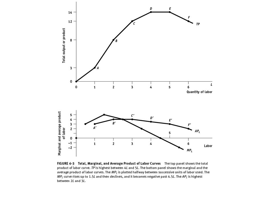
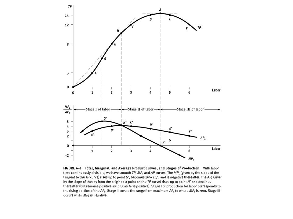
12. Production Function with One Variable Input
Total Product
TP = Q = f(L)
MPL =
TP L
Marginal Product
APL =
TP L
Average Product
EL =
MPL APL
Production or Output Elasticity

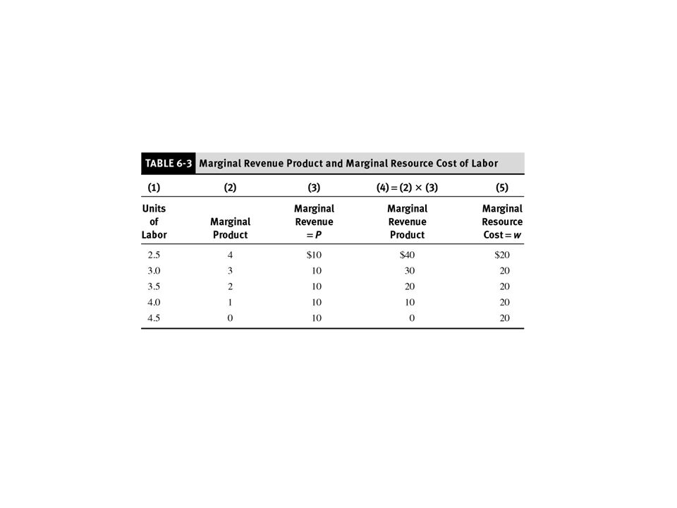
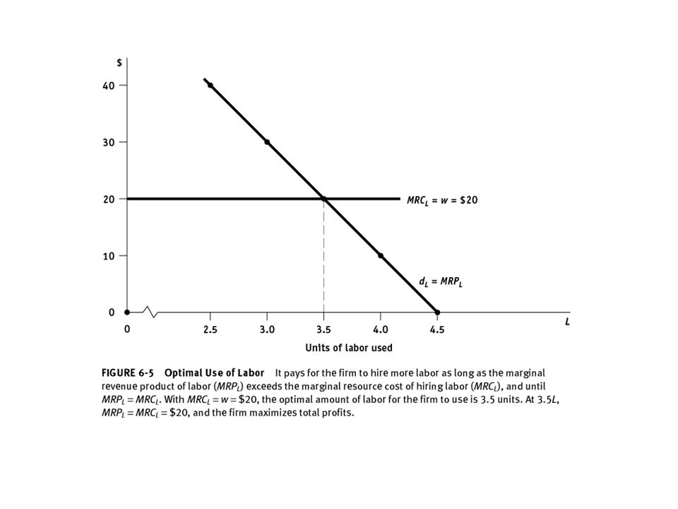
16. Optimal Use of the Variable Input
Marginal Revenue Product of Labor
MRPL = (MPL)(MR)
Marginal Resource Cost of Labor
TC L
MRCL =
Optimal Use of Labor
MRPL = MRCL

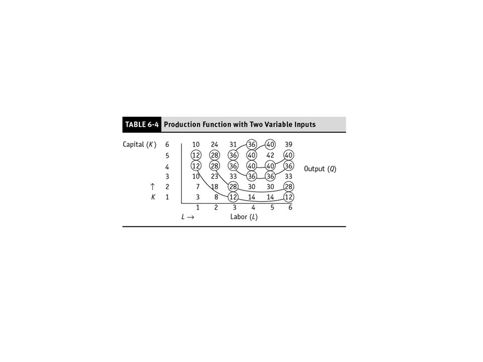
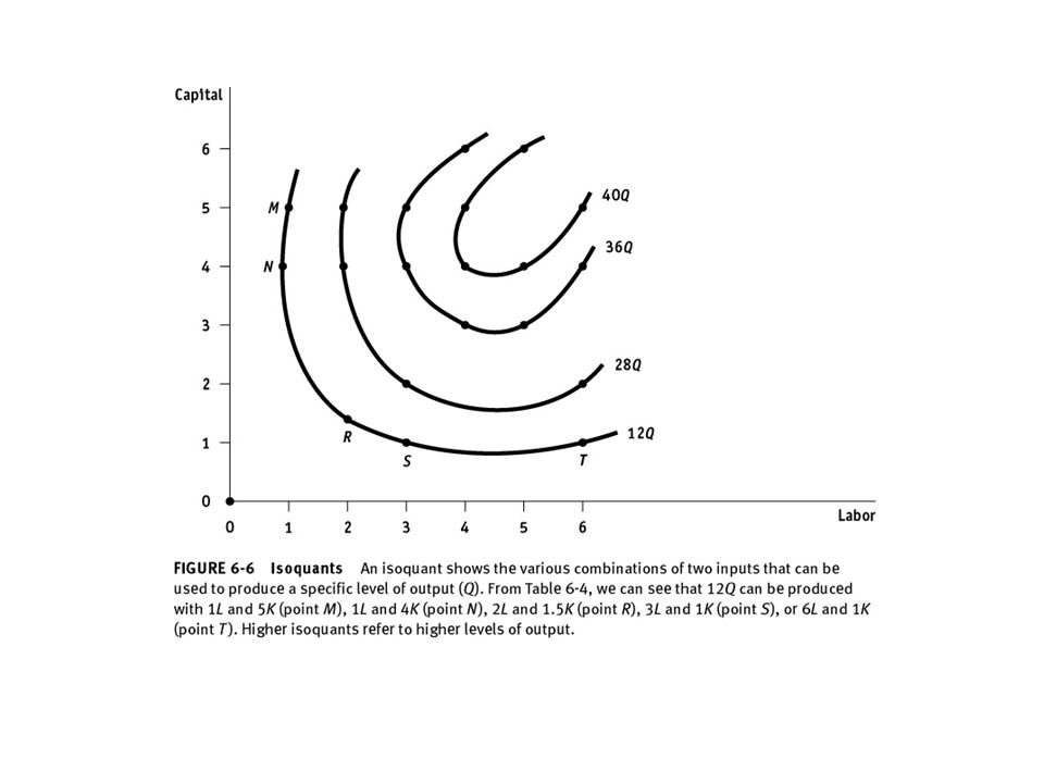
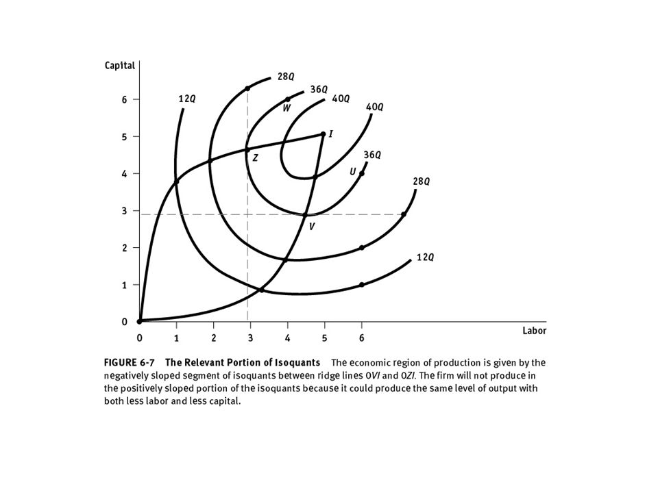
19. Production with Two Variable Inputs
Isoquants show combinations of two inputs that can produce the same level of output.
Firms will only use combinations of two inputs that are in the economic region of production, which is defined by the portion of each isoquant that is negatively sloped.

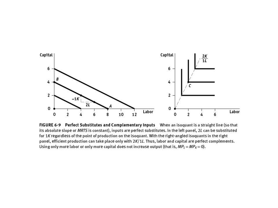
23. Isoquants When Inputs are Perfectly Substitutable
Capital
per
month Q1 Q2 Q3 A B C
Labor
per month 64

24. Production with Two Variable Inputs
Perfect Substitutes
Observations when inputs are perfectly substitutable:
1) The MRTS is constant at all points on the isoquant. 65

25. Production with Two Variable Inputs
Perfect Substitutes
Observations when inputs are perfectly substitutable:
2) For a given output, any combination of inputs can be chosen (A, B, or C) to generate the same level of output (e.g. toll booths & musical instruments) 65

26. Fixed-Proportions Production FunctionL1 K1 Q1 Q2 Q3 A B C
Capital
per
month
Labor
per month 66

27. Production with Two Variable Inputs
Fixed-Proportions Production Function
Observations when inputs must be in a fixed- proportion:
1) No substitution is possible.Each output requires a specific amount of each input (e.g. labor and jackhammers). 67

28. Production with Two Variable Inputs
Fixed-Proportions Production Function
Observations when inputs must be in a fixed- proportion:
2) To increase output requires more labor and capital (i.e. moving from A to B to C which is technically efficient). 67

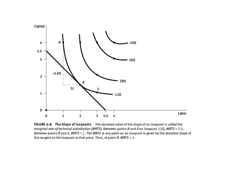
29. Production with Two Variable Inputs
Marginal Rate of Technical Substitution
MRTS = -K/L = MPL/MPK

31. Curves showing all possible combinations of inputs that yield the same output
An isoquant is a curve showing all possible combinations of inputs physically capable of producing a given fixed level of output
The isoquants emphasize how different input combinations can be used to produce the same output.
This information allows the producer to respond efficiently to changes in the markets for inputs.

32. Example 2 Production Table
Units of K
Employed
Isoquant

33. An Isoquant

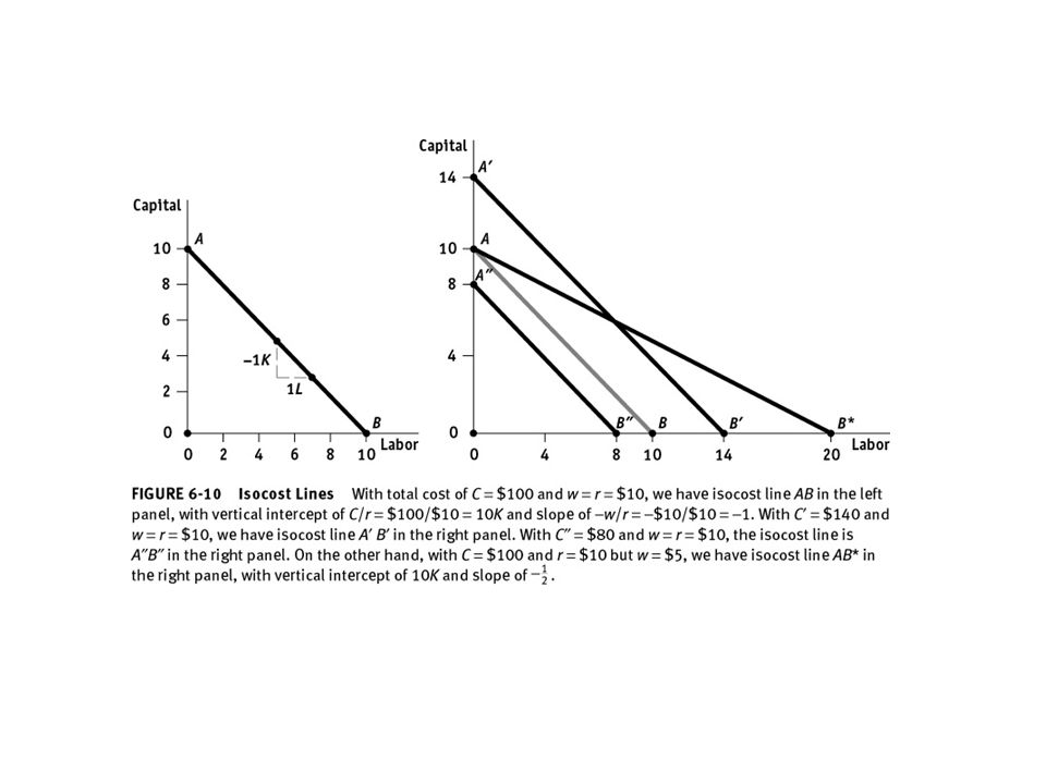
36. Isocost Line
Isocost line: shows all possible K/L combos that can be purchased for a given TC.
TC = C = w*L + r*K ;
Rewrite as equation of a line:
K = C/r – (w/r)*L
Slope = K/L = -(w/r).
Interpret slope:
* shows rate at which K and L can be traded off, keeping TC the same.
Relate to consumer’s budget constraint:
* slope = ratio of prices with price from horizontal axis in numerator.
Vertical intercept = C/r.
Horizontal intercept = C/w.

37. Units of Y 12 10 8 B = $1,000 B = $2,000 6 B = $3,000 4 2 Units of X 2
Production and Costs
Optimal combination of multiple inputs
Isocost curves.
All combinations of products
that can be purchased for a fixed
dollar amount
Units of Y 12 10
Downward sloping curve. 8 B
= $1,000 1
Shift B 2
= $2,000 6 B 3
= $3,000 4
Slope 2
Units of X 2 4 6

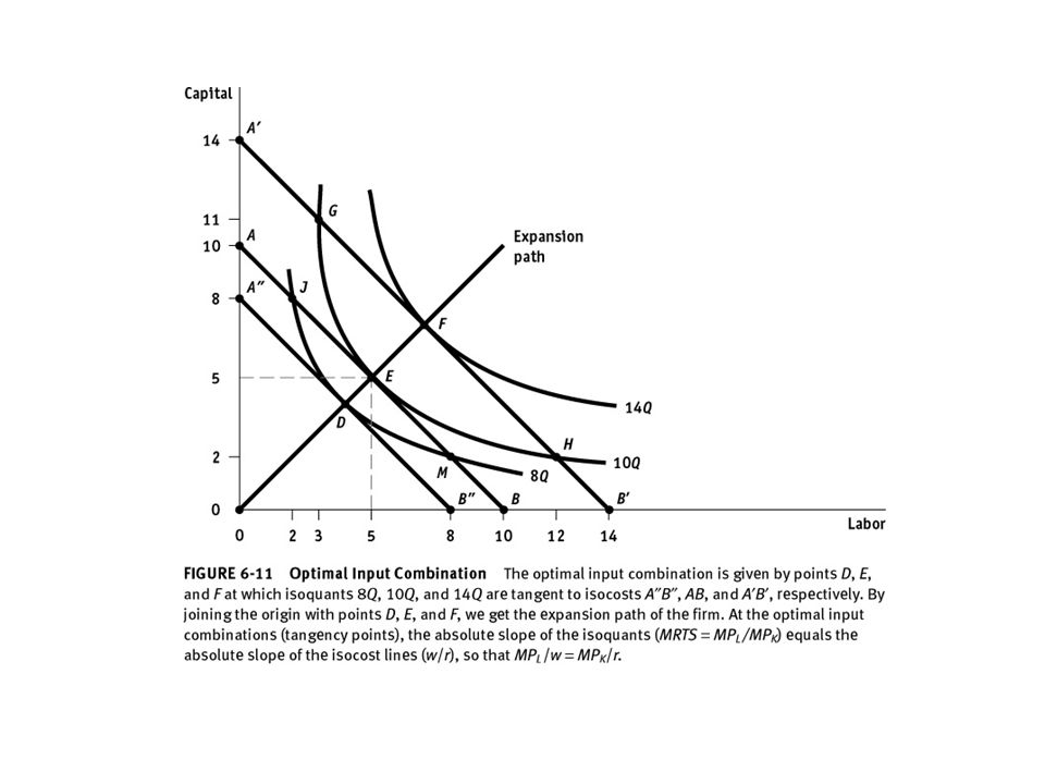
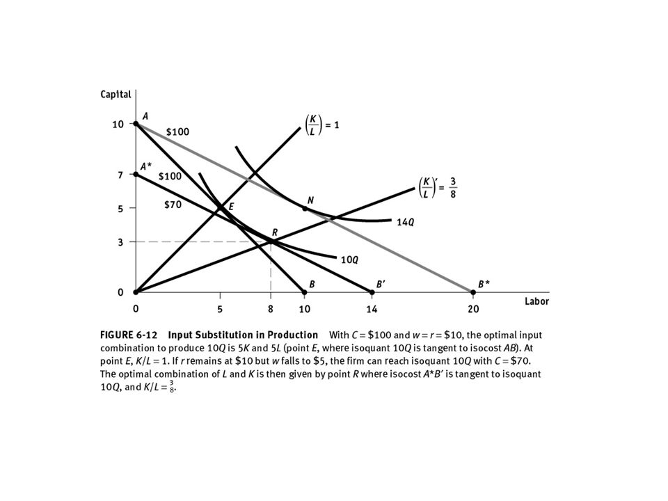
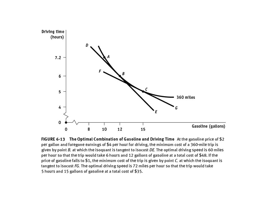
38. Optimal Combination of Inputs
Isocost lines represent all combinations of two inputs that a firm can purchase with the same total cost.

40. Optimal combination of multiple inputs
Production and Costs
Optimal combination of multiple inputs
Optimal combination corresponds to the point of tangency of the isoquant and isocost.
Units of Y B 3 B 2 B 1
Expansion path Y 3 C Y 2 B Y 1 A Q 3 Q 2 Q 1 X 1 X 2 X 3
Units of X

41. Optimal combination of multiple inputs
Production and Costs
Optimal combination of multiple inputs
Budget Lines
Least-cost production occurs when MPX/PX = MPY/PY and PX/PY = MPX/MPY
Expansion Path
Shows efficient input combinations as output grows.
Illustration of Optimal Input Proportions
Input proportions are optimal when no additional output could be produced for the same cost.
Optimal input proportions is a necessary but not sufficient condition for profit maximization.
Optimal combination corresponds to the point of tangency isoquant and isocost.
Units of Y B 3 B 2 B 1
Expansion path Y 3 Y 2 C Y B 1 A Q 3 Q 2 Q 1 X 1 X 2 X 3
Units of X

42. Optimal combination of multiple inputs
Production and Costs
Optimal combination of multiple inputs
Profits are maximized when MRPX = PX for all inputs.
Profit maximization requires optimal input proportions plus an optimal level of output.
Optimal combination corresponds to the point of tangency isoquant and isocost.
Units of Y B 3 B 2 B 1
Expansion path Y 3 Y 2 C Y B 1 A Q 3 Q 2 Q 1 X 1 X 2 X 3
Units of X

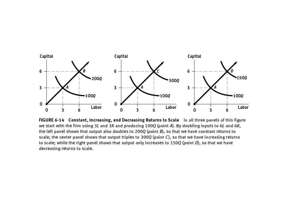
45. Production Function Q = f(L, K)
Returns to Scale
Production Function Q = f(L, K)
Q = f(hL, hK)
If  = h, then f has constant returns to scale.
If  > h, then f has increasing returns to scale.
If  < h, then f has decreasing returns to scale.

46. Returns to Scale
Measuring the relationship between the scale (size) of a firm and output
1) Increasing returns to scale: output more than doubles when all inputs are doubled
Larger output associated with lower cost (autos)
One firm is more efficient than many (utilities)
The isoquants get closer together 74

47. Returns to Scale Increasing Returns:
The isoquants move closer together 5 10 2 4 A
Capital
(machine
hours) 10 20 30
Labor (hours) 75

48. Returns to Scale
Measuring the relationship between the scale (size) of a firm and output
2) Constant returns to scale: output doubles when all inputs are doubled
Size does not affect productivity
May have a large number of producers
Isoquants are equidistant apart 76

49. Returns to Scale 10 20 30 15 5 10 2 4 A 6 Constant Returns:
Capital
(machine
hours) 15 5 10 2 4 A 6
Constant Returns:
Isoquants are equally spaced
Labor (hours) 75

50. Returns to Scale
Measuring the relationship between the scale (size) of a firm and output
3) Decreasing returns to scale: output less than doubles when all inputs are doubled
Decreasing efficiency with large size
Reduction of entrepreneurial abilities
Isoquants become farther apart 78

51. Returns to Scale 5 10 2 4 A 10 20 30 Decreasing Returns:
Capital
(machine
hours) 5 10 2 4 A 10 20 30
Decreasing Returns:
Isoquants get further
apart
Labor (hours) 75

52. Decreasing returns to scale
If an increase in all inputs in the same proportion k leads to an increase of output of a proportion less than k, we have decreasing returns to scale. Example: If we increase the inputs to a dairy farm (cows, land, barns, feed, labor, everything) by 50% and milk output increases by only 40%, we have decreasing returns to scale in dairy farming. This is also known as "diseconomies of scale," since production is less cheap when the scale is larger.
Constant returns to scale
If an increase in all inputs in the same proportion k leads to an increase of output in the same proportion k, we have constant returns to scale. Example: If we increase the number of machinists and machine tools each by 50%, and the number of standard pieces produced increases also by 50%, then we have constant returns in machinery production.
Increasing returns to scale
If an increase in all inputs in the same proportion k leads to an increase of output of a proportion greater than k, we have increasing returns to scale. Example: If we increase the inputs to a software engineering firm by 50% output and increases by 60%, we have increasing returns to scale in software engineering. (This might occur because in the larger work force, some programmers can concentrate more on particular kinds of programming, and get better at them). This is also known as "economies of scale," since production is cheaper when the scale is larger.

53. Determine the returns to scale of the following production functions:
1. F (z1, z2) = [z12 + z22]1/2.
2. F (z1, z2) = (z1 + z2)1/2.
3. F (z1, z2) = z11/2 + z2.
F (z1, 2) = [2z12 + 2z22]1/2 = (2)1/2(z12 + z22)1/2 = F (z1, z2). Thus this production function has CRTS.
F (z1, z2) = (z1 + z2)1/2 = 1/2(z1 + z2)1/2 = 1/2F (z1, z2). Thus this production function has DRTS.
F (z1, z2) = 1/2z11/2 + z2 < (z11/2 + z2) = F (z1, z2) for > 1. Thus this production function has DRTS

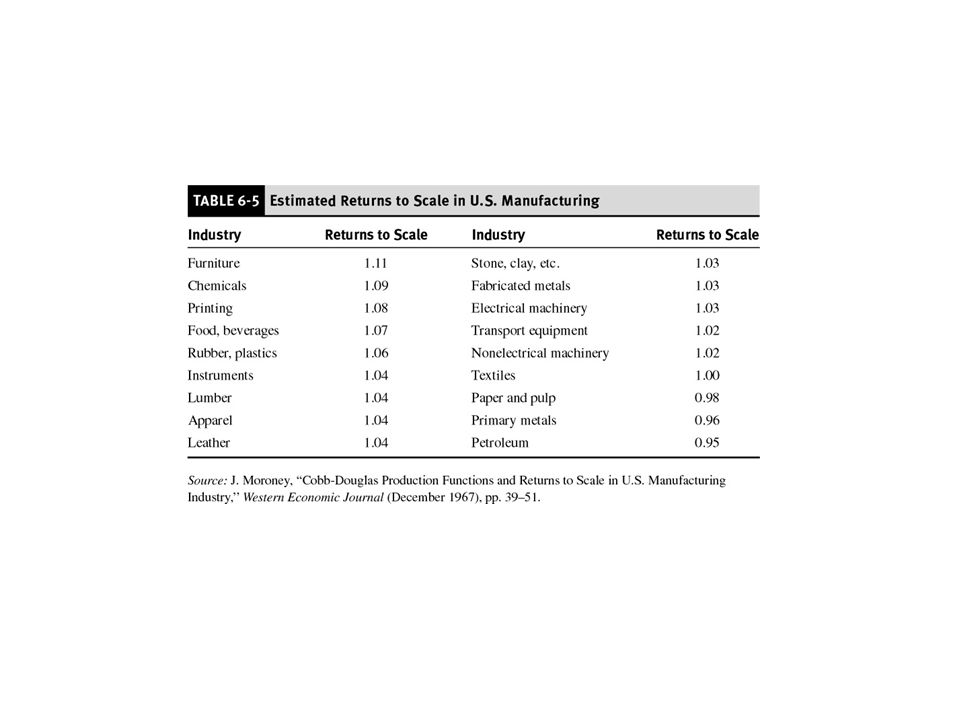
56. Empirical Production Functions
Cobb-Douglas Production Function
Q = AKaLb
Estimated Using Natural Logarithms
ln Q = ln A + a ln K + b ln L

57. Cobb-Douglas Production Function Example: Q = F(K,L) = K.5 L.5
K is fixed at 16 units.
Short run production function:
Q = (16).5 L.5 = 4 L.5
Production when 100 units of labor are used?
Q = 4 (100).5 = 4(10) = 40 units

58. Innovations and Global Competitiveness
Product Innovation
Process Innovation
Product Cycle Model
Just-In-Time Production System
Competitive Benchmarking
Computer-Aided Design (CAD)
Computer-Aided Manufacturing (CAM)
PowerPoint Slides Prepared by Robert F. Brooker, Ph.D. Slide 58