1. The free electron theory of metals The Drude theory of metals
Paul Drude (1900): theory of electrical and thermal conduction in a metal
application of the kinetic theory of gases to a metal,
which is considered as a gas of electrons
mobile negatively charged electrons are confined in a metal by attraction to immobile positively charged ions
isolated atom
nucleus charge eZa
Z valence electrons are weakly bound to the nucleus (participate in chemical reactions)
Za – Z core electrons are tightly bound to the nucleus (play much less of a role in chemical reactions)
in a metal – the core electrons remain bound to the nucleus to form the metallic ion
the valence electrons wander far away from their parent atoms
called conduction electrons or electrons
in a metal

2. Doping of Semiconductors
C, Si, Ge, are valence IV , Diamond fcc structure. Valence band is full
Substitute a Si (Ge) with P. One extra electron donated to conduction band
N-type semiconductor

3. density of conduction electrons in metals ~1022 – 1023 cm-3
rs – measure of electronic density
rs is radius of a sphere whose volume is equal to the volume per electron
mean inter-electron spacing
in metals rs ~ 1 – 3 Å (1 Å= 10-8 cm) rs/a0 ~ 2 – 6
Å – Bohr radius
● electron densities are thousands times greater than those of a gas at normal conditions
● there are strong electron-electron and electron-ion electromagnetic interactions
in spite of this the Drude theory treats the electron gas
by the methods of the kinetic theory of a neutral dilute gas

4. The basic assumptions of the Drude model
1. between collisions the interaction of a given electron
with the other electrons is neglected
and with the ions is neglected
2. collisions are instantaneous events
Drude considered electron scattering off
the impenetrable ion cores
the specific mechanism of the electron scattering is not considered below
3. an electron experiences a collision with a probability per unit time 1/τ
dt/τ – probability to undergo a collision within small time dt
randomly picked electron travels for a time τ before the next collision
τ is known as the relaxation time, the collision time, or the mean free time
τ is independent of an electron position and velocity
4. after each collision an electron emerges with a velocity that is randomly directed and
with a speed appropriate to the local temperature
independent electron approximation
free electron approximation

5. DC electrical conductivity of a metal
V = RI Ohm’s low
the Drude model provides an estimate for the resistance
introduce characteristics of the metal which are independent on the shape of the wire
j=I/A – the current density
r – the resistivity
R=rL/A – the resistance
s = 1/r - the conductivity L A
v is the average electron velocity

6. at room temperatures
resistivities of metals are typically of the order of microohm centimeters (mohm-cm)
and t is typically – s
mean free path l=v0t
v0 – the average electron speed
l measures the average distance an electron travels between collisions
estimate for v0 at Drude’s time → v0~107 cm/s → l ~ 1 – 10 Å
consistent with Drude’s view that collisions are due to electron bumping into ions
at low temperatures very long mean free path can be achieved
l > 1 cm ~ 108 interatomic spacings!
the electrons do not simply bump off the ions!
the Drude model can be applied where
a precise understanding of the scattering mechanism is not required
particular cases: electric conductivity in spatially uniform static magnetic field
and in spatially uniform time-dependent electric field
Very disordered metals and semiconductors

7. motion under the influence of the force f(t) due to spatially uniform
electric and/or magnetic fields
equation of motion
for the momentum per electron
electron collisions introduce a frictional damping term for the momentum per electron
average
momentum
average
velocity
Derivation:
fraction of electrons that
does not experience scattering
scattered
part
total loss of momentum
after scattering

8. Hall effect and magnetoresistance
Edwin Herbert Hall (1879): discovery of the Hall effect
the Hall effect is the electric
field developed across two
faces of a conductor
in the direction j×H
when a current j flows across
a magnetic field H
the Lorentz force
in equilibrium jy = 0 → the transverse field (the Hall field) Ey due to the accumulated charges
balances the Lorentz force
quantities of interest:
magnetoresistance
(transverse magnetoresistance)
Hall (off-diagonal) resistance
resistivity
Hall resistivity
the Hall coefficient
RH → measurement of the sign of the carrier charge
RH is positive for positive charges and negative for negative charges

9. force acting on electron equation of motion
for the momentum per electron
in the steady state px and py
satisfy
cyclotron frequency
frequency of revolution
of a free electron in the
magnetic field H
at H = 0.1 T
multiply by
the Drude
model DC
conductivity
at H=0
the resistance does not
depend on H
RH → measurement of the density
weak magnetic fields – electrons can complete only a small part of revolution between collisions
strong magnetic fields – electrons can complete many revolutions between collisions
j is at a small angle f to E f is the Hall angle tan f = wct

12. measurable quantity – Hall resistance
for 3D systems
for 2D systems n2D=n
in the presence of magnetic field the
resistivity and conductivity becomes tensors
for 2D:

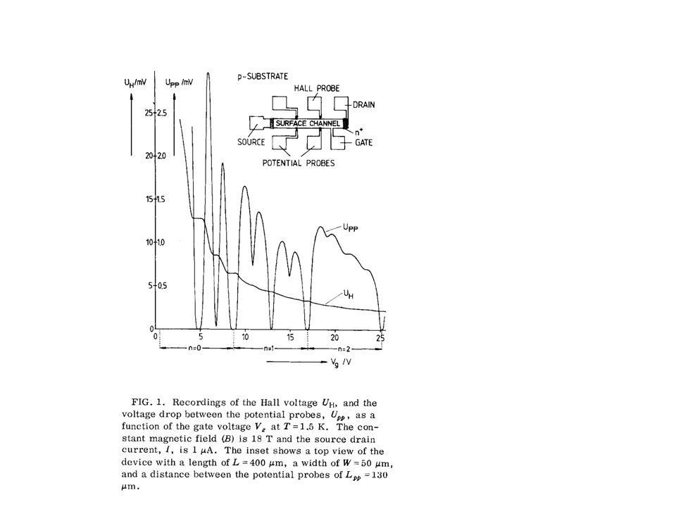
13. strong magnetic fields quantization of Hall resistance
weak
magnetic
fields
the Drude
model
the classical
Hall effect
strong magnetic fields
quantization of Hall resistance
at integer and fractional
the integer quantum Hall effect
and the fractional quantum Hall effect
from D.C. Tsui, RMP (1999) and from H.L. Stormer, RMP (1999)

14. AC electrical conductivity of a metal
Application to the propagation of electromagnetic radiation in a metal
consider the case
l >> l wavelength of the field is large compared to the electronic mean free path
electrons “see” homogeneous field when moving between collisions

15. response to electric field mainly historically
both in metals and dielectric described by used mainly for
electric current j conductivity s = j/E metals
polarization P polarizability c = P/E dielectrics
dielectric function e =1+4pc
electric field leads to
e(w,0) describes the collective
excitations of the electron
gas – the plasmons
e(0,k) describes the electrostatic
screening

16. AC electrical conductivity of a metal
equation of motion
for the momentum per electron
time-dependent electric field
seek a steady-state solution in the form
AC conductivity
DC conductivity
the plasma frequency
a plasma is a medium with positive
and negative charges, of which at
least one charge type is mobile

17. equation of motion of a free electron
even more simplified:
no electron collisions (no frictional damping term, )
equation of motion of a free electron
if x and E have the time dependence e-iwt
the polarization as the dipole moment per unit volume

18. Application to the propagation of electromagnetic radiation in a metal
transverse
electromagnetic
wave

19. Application to the propagation of electromagnetic radiation in a metal
electromagnetic wave equation
in nonmagnetic isotropic medium
look for a solution with
dispersion relation for
electromagnetic waves
(1) e real and > 0 → for w is real, K is real
and the transverse electromagnetic wave propagates
with the phase velocity vph= c/e1/2
(2) e real and < 0 → for w is real, K is imaginary
and the wave is damped
with a characteristic length 1/|K|:
(3) e complex → for w is real, K is complex
and the waves are damped in space
(4) e =  → The system has a final response in the
absence of an applied force (at E=0); the poles
of e(w,K) define the frequencies of the free
oscillations of the medium
(5) e = 0 longitudinally polarized waves are possible

20. Transverse optical modes in a plasma
dispersion relation for
electromagnetic waves
(1) for w > wp → K2 > 0, K is real,
waves with w > wp propagate in the media
with the dispersion relation
an electron gas is transparent
(2) for w < wp → K2 < 0, K is imaginary,
waves with w < wp incident on the medium
do not propagate, but are totally reflected
w/wp
(2) (1)
metals are shiny
due to the reflection
of light
w/wp
w = cK
electromagnetic waves are
totally reflected from the
medium when e is negative
electromagnetic waves
propagate without damping
when e is positive and real
forbidden
frequency gap
cK/wp
vph > c → vph does not correspond to the velocity of the real physical propagation of any quantity

22. Ultraviolet transparency of metals
plasma frequency wp and free space wavelength lp = 2pc/wp
range metals semiconductors ionosphere
n, cm
wp, Hz 5.7× × ×109
lp, cm 3.3× ×
spectral range UV IF radio
the reflection of
light from a metal
is similar to the
reflection of radio
waves from the
ionosphere
electron gas is transparent when w > wp i.e. l < lp
plasma frequency
ionosphere
semiconductors
metals
reflects transparent for
metal visible UV
ionosphere radio visible

23. Skin effect when w < wp electromagnetic wave is reflected
the wave is damped with a characteristic length d = 1/|K|:
the wave penetration – the skin effect
the penetration depth d – the skin depth
the classical skin depth
d >> l – the classical skin effect
d << l – the anomalous skin effect (for pure metals at low temperatures)
the ordinary theory of the electrical conductivity is no longer valid; electric field varies rapidly over l
not all electrons are participating in the absorption and reflection of the electromagnetic wave
only electrons that are running inside the skin depth for most of the mean
free path l are capable of picking up much energy from the electric field
only a fraction of the electrons d’/l are effective in the conductivity d’ l

24. Longitudinal plasma oscillations
a charge density oscillation, or
a longitudinal plasma oscillation, or plasmon
nature of plasma oscillations:
displacement of entire electron gas through d
with respect to positive ion background creates
surface charges s = nde and an electric field E = 4pnde
equation of
motion
oscillation at the
plasma frequency
for longitudinal plasma oscillation wL=wp
w/wp
transverse
electromagnetic waves
longitudinal plasma
oscillations
forbidden
frequency gap
cK/wp
equation of
continuity
for j~exp(-iwt)
Gauss’s law

25. Thermal conductivity of a metal
assumption from empirical observation - thermal current in metals is mainly carried by electrons
thermal current density jq – a vector parallel to the direction of heat flow
whose magnitude gives the thermal energy per unit time
crossing a unite area perpendicular to the flow
Fourier’s law
k – thermal conductivity
the thermal energy per electron
1D: to
3D:
high T low T
after each collision an electron emerges
with a speed appropriate to the local T
→ electrons moving along the T
gradient are less energetic
the electronic specific heat
Wiedemann-Franz law (1853)
Lorenz number ~ 2×10-8 watt-ohm/K2
Drude:
application of
classical ideal
gas laws
success of the Drude model is due to the cancellation
of two errors: at room T the actual electronic cv is 100
times smaller than the classical prediction, but v2 is 100
times larger

26. Thermopower
Seebeck effect: a T gradient in a long, thin bar should be accompanied by an electric field
directed opposite to the T gradient
high T low T
gradT E
thermoelectric field
thermopower
mean electronic velocity due to T gradient:
1D: to
3D:
mean electronic velocity due to electric field:
in equilibrium vQ + vE = 0 →
Drude:
application of
classical ideal
gas laws
no cancellation of two errors:
observed metallic thermopowers at room T are
100 times smaller than the classical prediction
inadequacy of classical statistical mechanics in describing the metallic electron gas

27. The Sommerfeld theory of metals
the Drude model: electronic velocity distribution
is given by the classical
Maxwell-Boltzmann distribution
the Sommerfeld model: electronic velocity distribution
is given by the quantum
Fermi-Dirac distribution
Pauli exclusion principle: at most one electron
can occupy any single electron level
normalization
condition T0

28. consider noninteracting electrons
electron wave function
associated with a level of energy E
satisfies the Schrodinger equation L
periodic
boundary
conditions
3D:
1D:
a solution neglecting
the boundary conditions
normalization constant: probability
of finding the electron somewhere
in the whole volume V is unity
energy
momentum
velocity
wave vector
de Broglie
wavelength

29. apply the boundary conditions components of k must be
the area
per point
the volume
k-space
apply the boundary conditions
components of k must be
nx, ny, nz integers
a region of k-space of
volume W contains
states
i.e. allowed
values of k
the number of states
per unit volume of k-space,
k-space density of states

30. the number of allowed values of k within the sphere of radius kF
consider T=0
the Pauli exclusion principle postulates that only one electron can occupy a single state
therefore, as electrons are added to a system, they will fill the states in a system
like water fills a bucket – first the lower energy states and then the higher energy states
the ground state of the N-electron system is formed by occupying all single-particle levels with k < kF
state of the lowest energy
volume
density
of states
the number of allowed values of
k within the sphere of radius kF kx ky kF
Fermi sphere
Fermi surface
at energy EF
to accommodate N electrons
2 electrons per k-level due to spin
Fermi wave vector ~108 cm-1
Fermi energy ~1-10 eV
Fermi temperature ~ K
Fermi momentum
Fermi velocity ~108 cm/s
compare to the ~ 107 cm/s at T=300K
classical
thermal velocity at T=0

31. density of states
total number of states with wave vector < k
total number of states with energy < E
the density of states – number of states per unit energy
the density of states per unit volume or the density of states
k-space density of states – the number of states per unit volume of k-space

32. Ground state energy of N electrons
add up the energies of all electron
states inside the Fermi sphere
volume of k-space per state
 smooth F(k)
the energy density
the energy per electron
in the ground state

33. remarks on statistics I
in quantum mechanics particles are indistinguishable
systems where particles are exchanged are identical
exchange of identical particles can lead to changing
of the system wavefunction by a phase factor only
repeated particle exchange → e2ia = 1
system of N=2 particles
x1, x2 - coordinates and
spins for each of the
particles
antisymmetric wavefunction with respect
to the exchange of particles
symmetric wavefunction with respect
to the exchange of particles
p1, p2 – single particle states
fermions are particles which have half-integer spin
the wavefunction which describes a collection
of fermions must be antisymmetric with respect
to the exchange of identical particles
fermions: electron, proton, neutron
bosons are particles which have integer spin
the wavefunction which describes a collection
of bosons must be symmetric with respect
to the exchange of identical particles
bosons: photon, Cooper pair, H atom, exciton
if p1 = p2 y = 0
→ at most one fermion can occupy
any single particle state – Pauli principle
unlimited number of bosons can occupy
a single particle state
obey Fermi-Dirac statistics
obey Bose-Einstein statistics

34. distribution function f(E) → probability that a state at energy E
will be occupied at thermal equilibrium
fermions
particles with
half-integer spins
bosons
integer spins
both fermions and
bosons at high T
when
Fermi-Dirac
distribution
function
Bose-Einstein
Maxwell-Boltzmann
degenerate
Fermi gas
fFD(k) < 1
Bose gas
fBE(k) can be any
classical
gas
fMB(k) << 1
m=m(n,T) – chemical potential

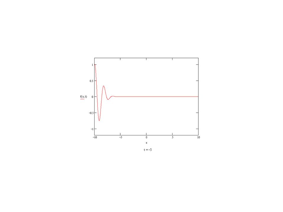
35. remarks on statistics IIv x
BE and FD distributions differ from the classical MB distribution because the particles they describe are indistinguishable.
Particles are considered to be indistinguishable if their wave packets
overlap significantly.
Two particles can be considered to be distinguishable
if their separation is large compared to their de Broglie wavelength. x
y(x)
vg=v
superposition of many waves Dx
g(k’) Dk k’
thermal de Broglie
wavelength
particles become
indistinguishable when
i.e. at temperatures below k0
A particle is represented by a
wave group or wave packets
of limited spatial extent,
which is a superposition of many matter waves with a spread of wavelengths centered on l0=h/p
The wave group moves
with a speed vg – the group speed,
which is identical to the classical
particle speed
Heisenberg uncertainty principle, 1927: If a measurement of position is made with precision Dx and a simultaneous measurement of momentum in the x direction is made with precision Dpx,
then
at T < TdB fBE and fFD are strongly different from fMB
at T >> TdB fBE ≈ fFD ≈ fMB
electron gas in metals:
n = 1022 cm-3, m = me → TdB ~ 3×104 K
gas of Rb atoms:
n = 1015 cm-3, matom = 105me → TdB ~ 5×10-6 K
excitons in GaAs QW
n = 1010 cm-2, mexciton= 0.2 me → TdB ~ 1 K

36. T≠0 the Fermi-Dirac distribution
density of states
distribution function
[the number of states in the energy range from E to E + dE]
[the number of filled states in the energy range from E to E + dE]
EF E
density of
filled states
D(E)f(E,T)
density of
states
D(E)
per unit volume
shaded area – filled
states at T=0

37. specific heat of the degenerate electron gas, estimate
T ~ 300 K for typical metallic densities
T = 0
specific heat
U – thermal
kinetic energy
f(E) at T ≠ 0 differs from f(E) at T=0
only in a region of order kBT about m
because electrons just below
EF have been excited to levels just above EF
classical gas
the observed electronic
contribution at room T is
usually 0.01 of this value
classical gas: with increasing T all electron gain an energy ~ kBT
Fermi gas: with increasing T only those electrons in states within
an energy range kBT of the Fermi level gain an energy ~ kBT
number of electrons which gain energy with increasing temperature ~
the total electronic thermal kinetic energy
the electronic specific heat
EF/kB ~ 104 – 105 K
kBTroom / EF ~ 0.01

38. specific heat of the degenerate electron gas
the way in which integrals of the form differ from their zero T values
is determined by the form of H(E) near E=m
replace H(E) by its Taylor expansion about E=m
the Sommerfeld expansion
successive terms are
smaller by O(kBT/m)2
for kBT/m << 1
replace m
by mT=0 = EF
correctly to order T2

39. specific heat of the degenerate electron gas
FD statistics depress
cv by a factor of
(1)
(2)

40. thermal conductivity
thermal current density jq – a vector parallel to the direction of heat flow
whose magnitude gives the thermal energy per unit time
crossing a unite area perpendicular to the flow
Wiedemann-Franz law (1853)
Lorenz number ~ 2×10-8 watt-ohm/K2
Drude:
application of
classical ideal
gas laws
success of the Drude model is due to the cancellation
of two errors: at room T the actual electronic cv is 100
times smaller than the classical prediction, but v is 100
times larger
for
degenerate
Fermi gas of
electrons
the correct at room T
the correct estimate of v2 is vF at room T

41. thermopower
Seebeck effect: a T gradient in a long, thin bar should be accompanied by an electric field
directed opposite to the T gradient
high T low T
gradT E
thermoelectric field
thermopower
Drude:
application of
classical ideal
gas laws
for
degenerate
Fermi gas of
electrons
the correct at room T
Q/Qclassical ~ at room T

42. Electrical conductivity and Ohm’s law
equation of motion
Newton’s law
in the absence of collisions the Fermi sphere in
k-space is displaced as a whole at a uniform rate
by a constant applied electric field
because of collisions the displaced Fermi sphere
is maintained in a steady state in an electric field
Ohm’s law ky F
kavg
Fermi sphere kx
the mean free path l = vFt
because all collisions involve only electrons near the Fermi surface
vF ~ 108 cm/s
for pure Cu:
at T=300 K t ~ s l ~ 10-6 cm = 100 Å
at T=4 K t ~ 10-9 s l ~ 0.1 cm
kavg << kF for n = 1022 cm-3 and j = 1 A/mm2 vavg = j/ne ~ 0.1 cm/s << vF ~ 108 cm/s