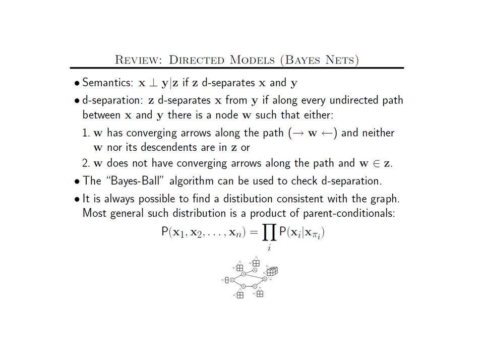
1. P(h i ) is called the hypothesis prior Nothing special about “learning” – just vanilla probabilistic inference

2. Where is the hypothesis prior?

3. How did this prediction come about? Which hypothesis did we use?

4. The analogy with diagnosis Medical diagnosis Given symptoms of a patient, predict whether she will have other symptoms (such as death…) Can try predicting directly from symptoms (is what we did before the advent of medicine) But we normally assume that diseases cause symptoms.. Thus we want to first figure out the disease and then predict other symptoms Diseases have prior probabilities (in fact, the “ignored prior” fallacy is the main reason for internet induced hypochondria) Given the symptoms, we compute the posterior on the diseases, and then use that to predict other symptoms Full Bayesian learning Given training data, predict test data Can try predicting test data directly from training data (e.g. k-NN) But we normally assume that hypothesis explain data. Thus we want to first figure out the hypotheses causing the data and then using them predict test data Hypotheses have prior probabilities (as to how likely they are— independent of the data being seen right now). Given the data, we compute the posterior on the hypotheses, and then use that to predict test data

5. 11/15

6. Density Estimation (as the general objective of Statistical Learning) Given data D whose instances are made-up of attributes  that are distributed according to P*(  ), we want to learn an estimate P’ to P* such that the distance between P* and P’ is minimized Once we have P’, we can use it for (i) prediction (ii) completion (iii) generation We need to decide how to represent P’ – We shall assume graphical models Bayes Networks or Markov Networks Often  can be partitioned into X (the “input attributes”) and Y (the “output attributes”) – In such a case, rather than learn P*(  ), we might want to learn P*(Y|X) – If we do this, then we are doing discriminative learning (as against generative learning)

7. P(h i ) is called the hypothesis prior Nothing special about “learning” – just vanilla probabilistic inference Note that for density Estimation, H is the Density and P(H) is the Density over densities!  For parametric case P(H) would be a distribution Over the parameters E.g. If we believe that the Hypothesis is a normal Distribution, then P(H) is a distribution over mean And variance of the normal  For non-parametric case things are much harder as you need the P(H) to be A distribution over infinite parameters (the recent advances on gaussian processes are aimed at this) Two problems: 1. need to represent P(H) during learning 2. Need to reason with P(H) during inference MAP does away with 2 while MLE does away With both 1 and 2

8. How many Why should P(h i ) be low for complex hypotheses? --connection to MDL principle Equivalently minimize - log P(d|h i ) – log P(h i ) Bits required to specify h i Additional bits required to specify d Need to represent both P(x|h) and P(h|D) We can no longer quantify the variance of our prediction  What if h MAP is just a little more likely than the next best and they predict different results?

9. --because “statisticians” distrust priors (and want the data to speak for itself) When will ML hit roadblock? Small data Not only can’t we quantify the variance of our prediction, but we also can fall prey to over fitting  For example, the likelihood of data will never reduce if we add more links into the bayes network. So we will wind up learning fully connected networks!

10. Density Estimation The general task of learning a probability model, given data that are assumed to be generated from that model Given data D whose instances are made-up of attributes  that are distributed according to P*(  ), we want to learn an estimate P’ to P* such that the distance between P* and P’ is minimized – Distance between distributions is typically measured using KL Divergence – D(P*||P’) = E P* [log P*(  )/P’(  )] But alas, we don’t know P*  = E P* log P*(  ) - E P* log P’(  ) The first term is constant and can be ignored in comparing two estimates P’ and P’’ But how do we get the second term? Since the data instances are drawn from P*, a P’ that maximizes their log likelihood is the best. If data are drawn i.i.d, then their joint likelihood is a product and log terms over all data instances can be summed..

11. Bias-Variance Tradeoff (learning with bias vs. regularization) So, we want to get the distribution P’ that maximizes E P* log P’(  ) – Learning is just optimization! But how do we select the candidate space of distributions (hypotheses)? [Bias problem] If the class of distributions we consider is too small/inflexible (“highly biased”), then the best we get may still be too far from P* [Variance problem] If the class of distributions considered is too large/expressive, then small random fluctuations in the choice of data can radically change the properties of the model, thus exhibiting high variance on the test data Standard solutions: 1.Limit attention to a “reasonable class of distributions” (e.g. Naïve Bayes) 2.Allow a large class of distributions, but “penalize” the more complex ones [Also called “regularization”]. 3.Combination of both.. A class of distributions can be defined by restricting the class of graphical models (e.g. only naïve bayes models) or CPDs (only noisy-or or conditional Gaussians) allowed in the hypothesis space

12. Generative vs. Discriminative Learning Often, we are really more interested in predicting only a subset of the attributes given the rest. – E.g. we have data attributes split into subsets X and Y, and we are interested in predicting Y given the values of X You can do this by either by – learning the joint distribution P(X, Y) [Generative learning] – or learning just the conditional distribution P(Y|X) [Discriminative learning] Often a given classification problem can be handled either generatively or discriminatively – E.g. Naïve Bayes and Logistic Regression Which is better?

13. Bayesians vs. Frequentists (The Religious Wars) Frequentist Learning Probabilities are “asymptotic frequencies” There is a TRUE hypothesis – So Hypothesis is not a random variable; and can’t have a distribution Having a prior is like “cheating”; being prejudiced; – Let the data speak for itself! Bayesian Learning Probabilities are “degrees of beliefs” Hypothesis is a random variable So can have a prior and a posterior The hypothesis Prior is the agent’s belief about which hypotheses are more vs. less likely Probability that Einstein drank a cup of tea at 4:13pm on Feb 26, 1920? “I believe it is 0.4” Can’t say! God Doesn’t Play dice with the universe Stop telling God what to do! Both camps agree on MLE (but for differrent reasons) MLE is just stripped down special case of Bayesian Learning for large data Good that you got out of hypothesis prior. Just don’t say P(D|h); it is P(D; h) you know..

14. http://web.mit.edu/cocosci/Papers/significance.pdf Should AI also distrust priors? Priors can encode background knowledge.. (There is evidence that human brain uses priors)

15. Density Estimation (as the general objective of Statistical Learning) Given data D whose instances are made-up of attributes  that are distributed according to P*(  ), we want to learn an estimate P’ to P* such that the distance between P* and P’ is minimized Once we have P’, we can use it for (i) prediction (ii) completion (iii) generation We need to decide how to represent P’ – We shall assume graphical models Bayes Networks or Markov Networks Often  can be partitioned into X (the “input attributes”) and Y (the “output attributes”) – In such a case, rather than learn P*(  ), we might want to learn P*(Y|X) – If we do this, then we are doing discriminative learning (as against generative learning)

16. Generative vs. Discriminative Generative Learning More general (after all if you have P(Y, X) you can predict Y given X as well as do other inferences – You can predict jokes as well as make them up (or predict spam mails as well as generate them) In trying to learn P(Y,X), we are often forced to make many independence assumptions both in Y and X—and these may be wrong.. – Interestingly, this type of high bias can help generative techniques when there is too little data Discriminative Learning More to the point (if what you want is P(Y|X), why bother with P(Y,X) which is after all P(Y|X) *P(X) and thus models the dependencies between X’s also? Since we don’t need to model dependencies among X, we don’t need to make any independence assumptions among them. So, we can merrily use highly correlated features.. – Interestingly, this freedom can hurt discriminative learners when there is too little data (as over fitting is easy) P(y)P(x|y) = P(y,x) = P(x)P(y|x)

17. Dimensions of Statistical Learning Tasks Model constraints Type of network being learned – Bayes Network vs. Markov network Topology given; CPTs to be learned Only relevant attributes are given; need to learn topology as well as CPTs – Tricky part for MLE is that increasing the connectivity of a network cannot reduce likelihood We don’t know what the relevant attributes are Observability of data Complete data – Each data instance gives the values of each of the attributes Incomplete data – Some of the data instances might be missing the values for some of the attributes Hidden attributes (variables) – None of the data instances have values for some of the attributes (which often correspond to “intermediate” concepts which help improve the sparsity of network. E.g. “syndromes” which connect symptoms to diseases; or class variables in mixture models Sample complexity linearly varies with # parameters to be learned, and #parameters vary exponentially with # edges in the graphical model Philisophy of learning Bayesian Keep a distribution over hypotheses MAP Keep just the best hypothesis (that has the highest prior + likelihood) MLE Keep just the hypothesis that maximizes likelihood

18. Our Agenda We shall focus on density estimation tasks and consider generative case first We will focus on Bayes Networks first (and time permitting, Markov Networks) We will focus on MLE learning first (and then full bayesian learning) We will focus on complete data first; and then incomplete data and/or hidden variables

20. Steps in ML based learning 1.Write down an expression for the likelihood of the data as a function of the parameter(s)  Assume i.i.d. distribution 2.Write down the derivative of the log likelihood with respect to each parameter 3.Find the parameter values such that the derivatives are zero  There are two ways this step can become complex  Individual (partial) derivatives lead to non-linear functions (depends on the type of distribution the parameters are controlling; binomial is a very easy case)  Individual (partial) derivatives will involve more than one parameter (thus leading to simultaneous equations) In general, we will need to use continuous function optimization techniques One idea is to use gradient descent to find the point where the derivative goes to zero. But for gradient descent to find global optimum, we need to know for sure that the function we are optimizing has a single optimum (this is why convex functions are important. If the likelihood is a convex function, then gradient descent will be guaranteed to find the global minimum).

21. Note that for us, data are 2-attribute tuples [Flavor, Wrapper]

22. No entanglement of parameters for complete data for Bayes nets with known topology and tabular CPTs Specifically, each partial derivative will involve only one parameter i.e., each partial derivative contains only one parameter so you are solving single variable equations rather than simultaneous equations.  doesn’t hold for markov nets  ; doesn’t also hold for Bayes nets where CPDs induce direct parameter dependencies

23. Celebrating ease of learning for bayes nets with complete data! So we just noted that if we know the topology of the Bayes net, and we have complete data then the parameters are un-entangled, and can be learned separately from just data counts. Questions: How big a deal is this? – Can we have complete data? – Can we have known topology?

24. Learning the parameters for Continuous Case (Gaussian Distribution)

25. i.i.d. assumption

26. Problems with ML and Bayesian Learning.. ML based learning is unable to take the size of the data into account (1/3 is the same as 1M/3M) We however tend to start with a prior, and are less willing to change the prior unless shown enough evidence – Bayesian learning can handle this.. If a thumbtack came up heads once when you tossed it 3 times, what is the probability that it will come up heads the next time? Now, a coin came up heads once when you tossed it heads three times. What do you think is the probability that it will come up heads next time? How about if it came up heads 1million times in 3 million trials?

27. Bayesian Learning (for coin toss..) Let  be the probability that the coin comes heads – Each different value of  is a different hypothesis – So P(h) –the hypothesis prior– can be specified by specifying P(  ) Starting with prior on  we just need to compute the posterior Challenge: Find a distribution over continuous space that – can be represented compactly – And keeps its form upon update.. Example: Uniform; but what if we have a more information? Beta distributions – Think of a and b as the number of heads and tails you have seen prior to the start of this experiment – Update: head

28. “Conjugate Prior” A prior distribution family P c is considered a conjugate prior for a likelihood function family P l if starting with a hypothesis prior P c 1 from P c and seeing data with likelihood P l from P l the posterior of the hypothesis prior will also be in P c – Beta distributions are conjugate priors for bernouli (Binomial) likelihood distributions – Dirichlet distributions are conjugate priors for Multinomial likelihood distributions – Normal-Wishart distributions are conjugate priors for Gaussian likelihood distributions

29. Bayesian Prediction So suppose we started with Beta[a,b] as the prior – Probability of heads will be a/(a+b) If you manage to evaluate ∫ P(heads|  )P(  ) d  Now after seeing D h heads and D t tails, the posterior will be Beta[a+D h, b+D t ] – Probability of heads now will be (a+D h )/(a+D h + b+D t ) So, to the ML estimate, you just add a + b virtual samples… – Is what you did with Laplace Smoothing… Laplace smoothing is a backdoor way of making ML predictions be in line with full Bayesian learning…

30. Multi-parameter case (Assume Parameter Independence) Each example is “inserted” Into the bayes network as evidence and posterior over parameters is queried The wrench in the works Is that the size of the Network grows with examples(!) and we have Continuous quantities For table CPDs, Prior should be a dirichlet Distribution Notice that we assumed Parameter Independence Dirichlet Prior

31. Priors and Background Knowledge Hypothesis priors can be seen as providing background knowledge Background knowledge is also helpful in “logical learning” – Sao Paulo airport example

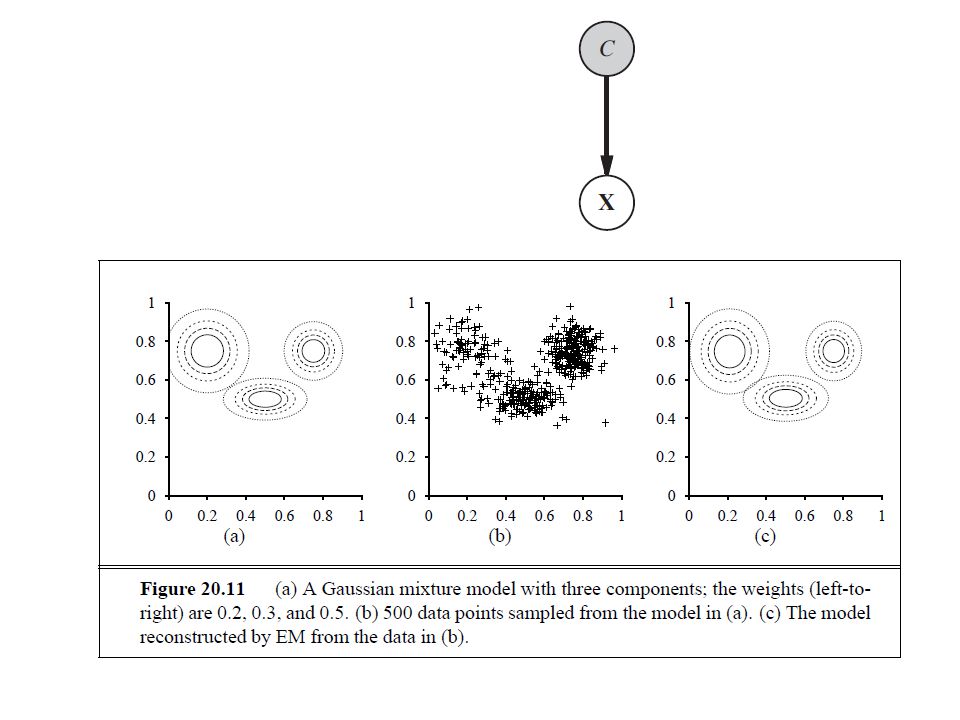
33. Case Study: Learning Bayes Net models for Relational database tables Consider a relational table in RDBMS with n attributes – Say an employee table giving the age, position, salary etc of each employee Suppose we want to learn the generative model underlying it Suppose we were able to hypothesize the topology – We might be able to do so if (a) we know the domain or (b) we know some of the causal dependencies in the data If the relational table is “complete” –i.e.., every tuple gives the value for every attribute, (which is the standard RDBMS model), then learning the parameters of this network is easy! Now, suppose the table is slightly “dirty”—in that there are tuples that have some missing values for some of the attributes – Say, some of the employee tuples are missing age information, others are missing salary information etc. If only a small percent of the tuples are incomplete, then we can – 1. Learn the model using the complete tuples – 2. predict the null values in the dirty tuples using the learned model But, if a non-trivial percent of the tuples are incomplete, then, we might want to continue for step 2 above by – 3. Now that we have “completed” all the incomplete tuples, we have fully complete data. Learn the model with this Completed data; and see if it is any better A model is better if it provides a higher likelihood for the observed data But why stop here? Continue and use the new model to re-predict the missing values, and iterate – This is the basic idea of EM (Expectation Maximization) algorithm

34. What if the best generative model contains attribute that are not mentioned in the table? In the previous relational table scenario, we assumed that some of the tuples are missing some of the attribute values. What if all tuples are missing some attribute values? – E.g. Educational level of the employee can be an attribute that is missing in the current table. This is like having an attribute column whose value is not known for any of the tuples – Why would we do it? – Can we still use EM? Can we still use EM? – Surprisingly, it turns out yes. In the earlier scenario, we used the complete tuples for setting up the initial model, but then used it to complete the data, and loop – There is no reason why we should initialize using complete data. We can initialize the model (parameters) randomly, and still do the EM looping! But why would we do it? – Given a complete relational table, such as the employee one, why would we start hypothesizing hidden attributes? – Because the right hypothesis on the hidden attribute can significantly reduce the number of parameters – For example, the educational level of the employee might cluster employees into “PhD” folks (who presumably have high salaries, interesting positions, and mature ages), and “non-PhD” folks (who presumably have low salaries, green-behind-the-ears ages, and assembly programming kind of jobs), and in each cluster the distributions of the attribute values are different (as described above) So, – Hypothesizing hidden attributes reduces the parameters to be estimated, but makes their estimation hard – Not hypothesizing them allows us to deal with complete data, but might require exponentially many parameters to be learned (from the same data—making the parameters, while easy to estimate, pretty worthless in terms of accuracy.

35. The “size of the step” is determined adaptively by where the max of the lowerbound is.. --In contrast, gradient descent requires a stepsize parameter --Newton Raphson requires second derivative.. Why does EM Work? Log of Sums don’t have easy closed form optima; use Jensen’s inequality and focus on Sum of logs which will be a lower bound F t (J) is an arbitrary prob dist over J By Jensen’s inequality

37. Missing data (but no hidden variables)

38. Involves Bayes Net inference; can get by with approximate inference Involves maximization; can get away with just improvement (i.e., a few steps of gradient ascent)

39. Where P(Xj|Ci) can be any distribution…

43. 0. Initialize the parameters randomly Loop Inference

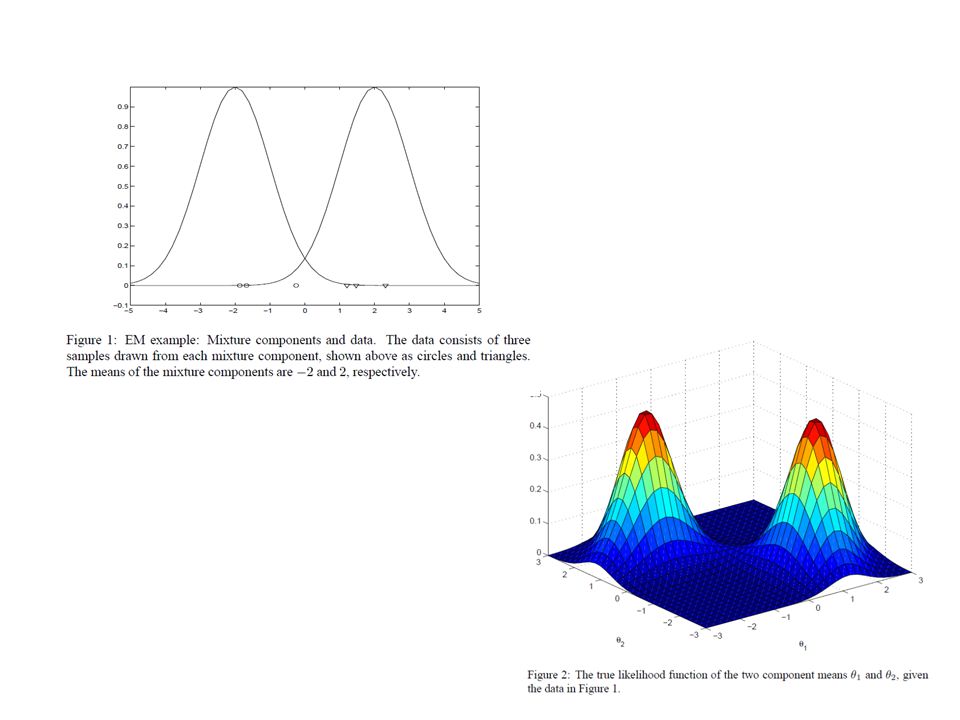
44. Why is hidden variable case hard? We need to compute log likelihood by marginalizing over hidden variables By Jensen’s inequality

45. Candy Example Start with 1000 samples Initialize parameters as

46. Jensen’s inequality generalizes the convexity definition of a function

50. Structure (Topology) Learning Search over different network topologies Question: How do we decide which topology is better? – Idea 1: Check if the independence relations posited by the topology actually hold – Idea 2: Consider which topology agrees with the data more (i.e., provides higher likelihood) But need to be careful--increasing edges in a network cannot reduce likelihood – Idea 3: Need to penalize complexity of the network (either using prior on network topologies, or using syntactic complexity measures)

51. Structure learning with BIC/MDL Scores Dim(G) is the number of free parameters in the model  The denser the connections, the higher dim(G)  The more structured the CPTs the lower dim(G)

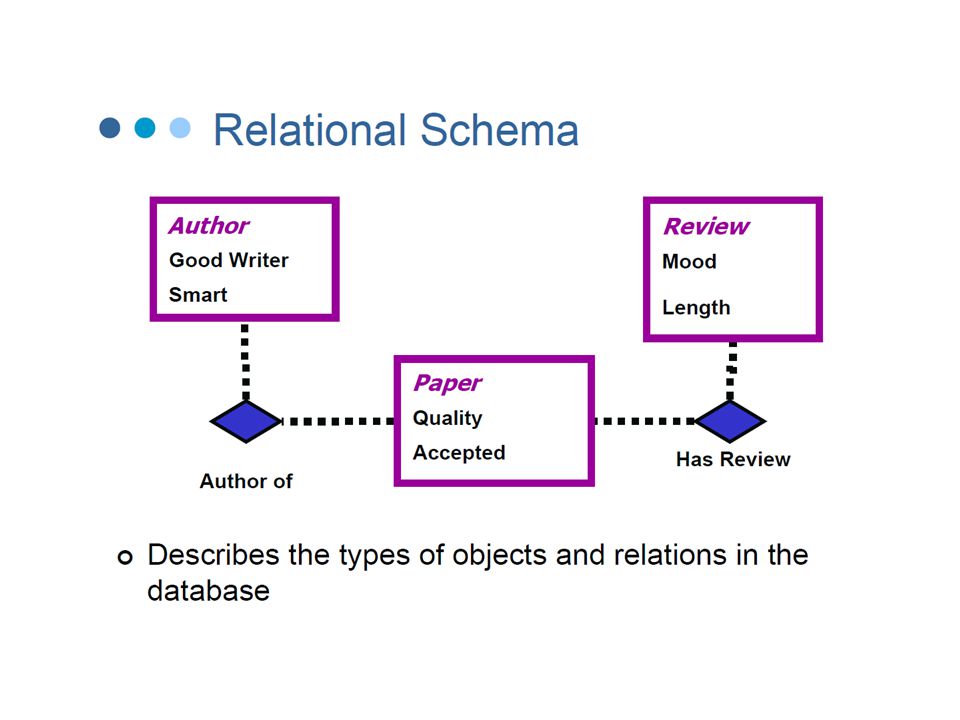
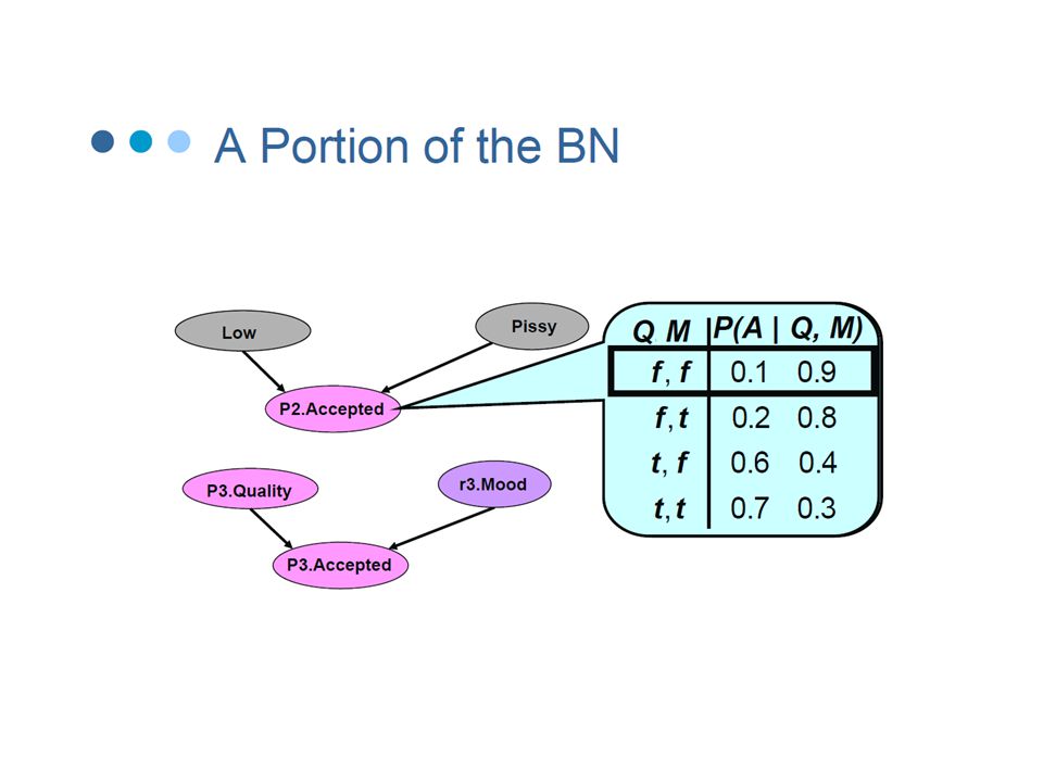
53. Relational Probabilistic Models Bayes nets are “propositional” models. We will now look at a generalization of bayes nets to “relational” case –..where the world is made up of objects and relations between them –..think predicate logic (not First order though..)

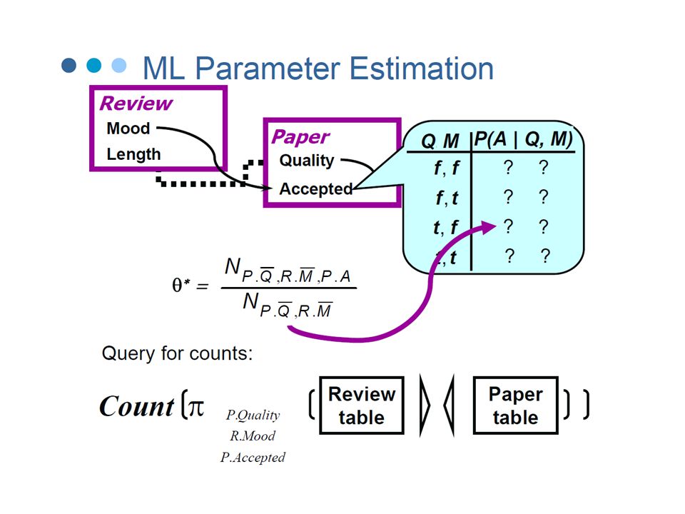
58. Note that we are assuming the same CPT Holds for ALL authors/papers/reviews --A tremendous saving in parameters

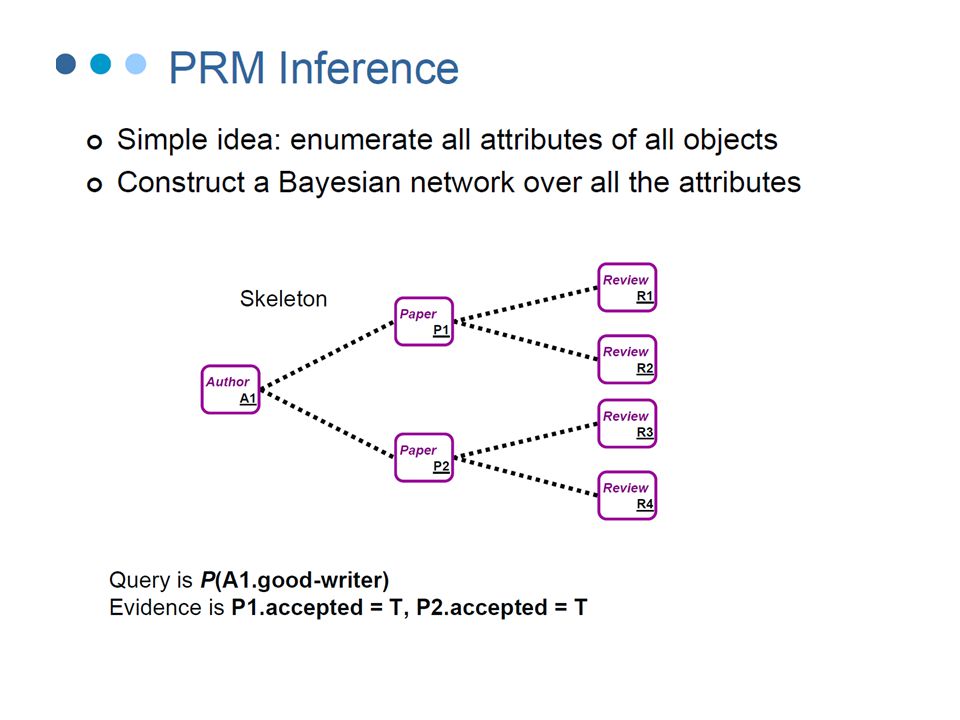
64. Sort of like propositional semantics for predicate logic…

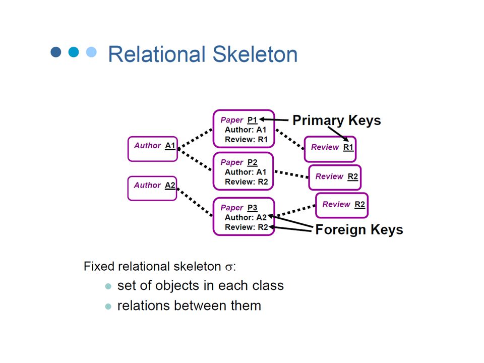
65. PRMs vs. Bayes Nets The semantics of PRMs are in terms of the underlying bayes nets However, – The PRM defines the dependencies at the class level rather than at the object level..and these dependencies and CPTs are used for all objects of that class – The PRM allows dependencies between the attributes of different objects (e.g. review’s mood affects paper’s decision)

67. Sort of like doing predicate logic inference by compiling to propositional logic

68. Need lifted inference techniques

70. Note that the author of the paper doesn’t matter since we assume the CPT is the same for all papers --Significant sample efficiency

72. --Slides beyond this not covered--

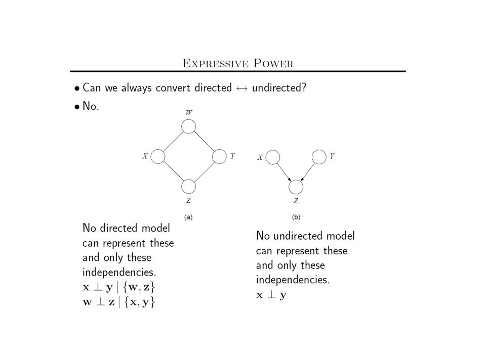
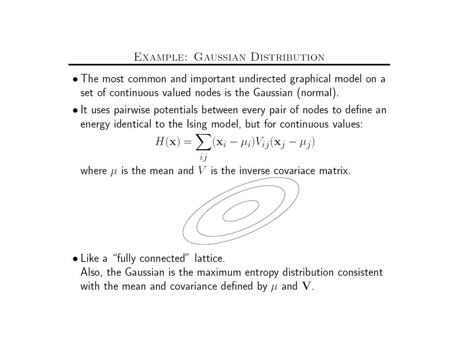
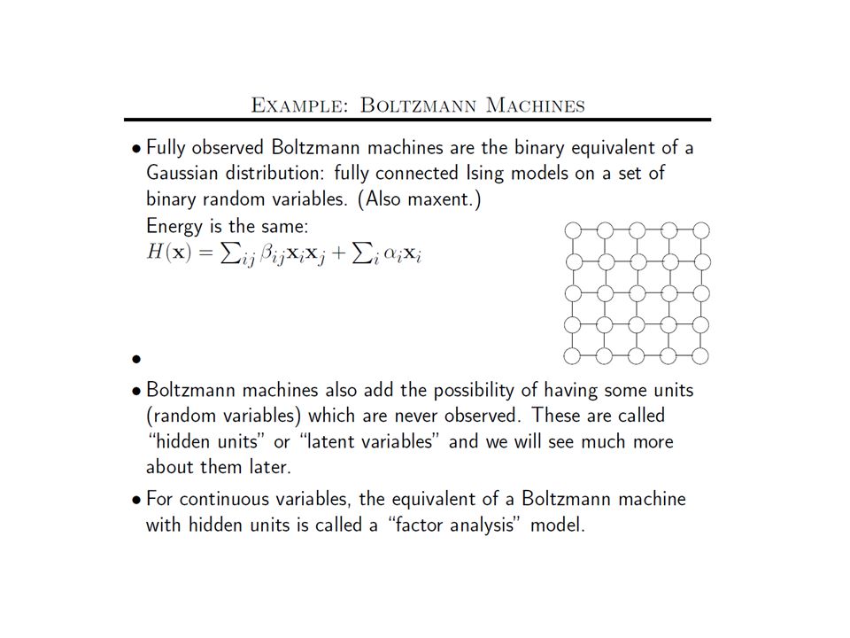
73. Undirected Probabilistic Graphical Models (Markov Nets) (Slides from Sam Roweis Lecture)

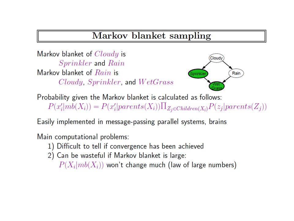
78. Connection to MCMC:  MCMC requires sampling a node given its markov blanket  Need to use P(x|MB(x)). For Bayes nets MB(x) contains more nodes than are mentioned in the local distribution CPT(x)  For Markov nets,

79.  Because neighbor relation is symmetric nodes xi and xj are both neighbors of each other..

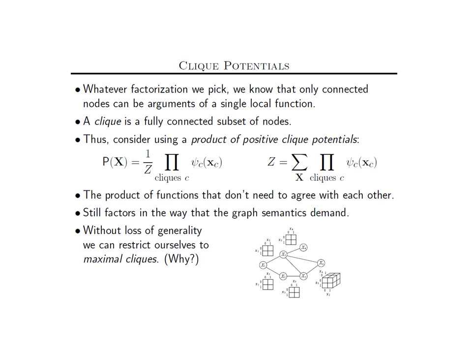
83. Markov Networks Undirected graphical models Cancer CoughAsthma Smoking Potential functions defined over cliques SmokingCancer Ф(S,C) False 4.5 FalseTrue 4.5 TrueFalse 2.7 True 4.5

85. Markov Networks Undirected graphical models Log-linear model: Weight of Feature iFeature i Cancer CoughAsthma Smoking

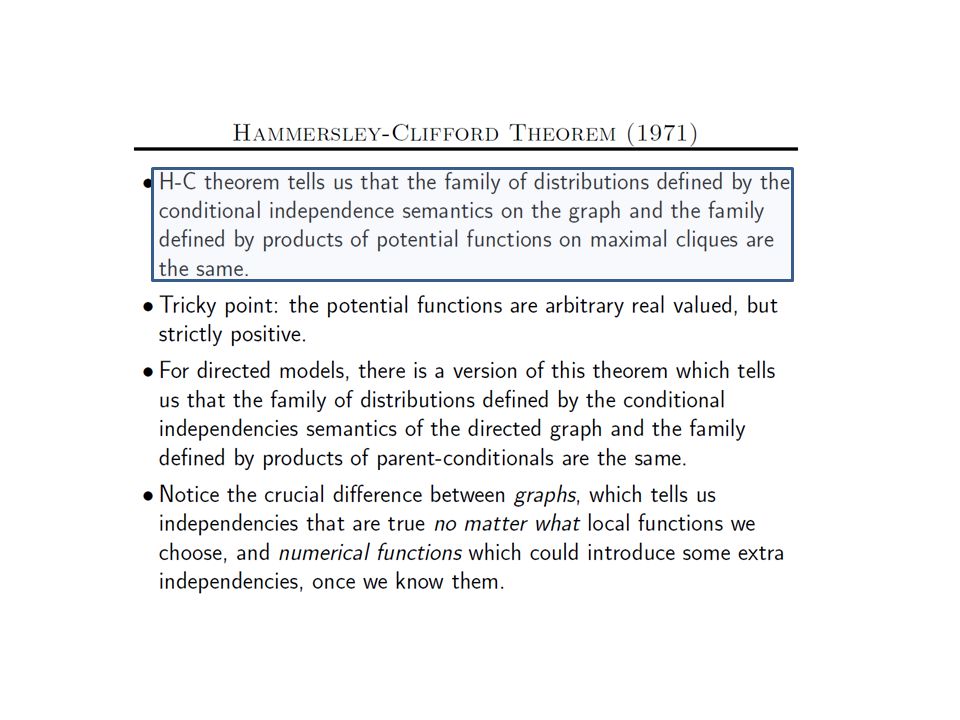
89. Hammersley-Clifford Theorem If Distribution is strictly positive (P(x) > 0) And Graph encodes conditional independences Then Distribution is product of potentials over cliques of graph Inverse is also true. (“Markov network = Gibbs distribution”)

94. Markov Nets vs. Bayes Nets PropertyMarkov NetsBayes Nets FormProd. potentials PotentialsArbitraryCond. probabilities CyclesAllowedForbidden Partition func.Z = ? globalZ = 1 local Indep. checkGraph separationD-separation Indep. props.Some InferenceMCMC, BP, etc.Convert to Markov

96. Inference in Markov Networks Goal: Compute marginals & conditionals of Exact inference is #P-complete Conditioning on Markov blanket is easy: Gibbs sampling exploits this Partition function cancels out

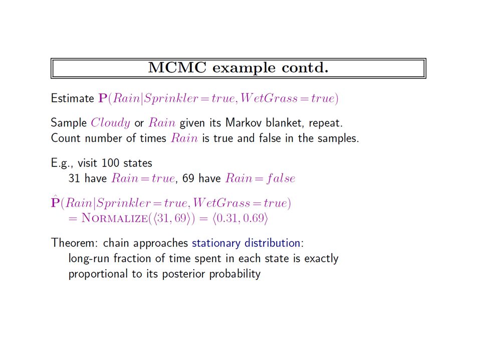
100. MCMC: Gibbs Sampling state ← random truth assignment for i ← 1 to num-samples do for each variable x sample x according to P(x|neighbors(x)) state ← state with new value of x P(F) ← fraction of states in which F is true

101. Other Inference Methods Many variations of MCMC Belief propagation (sum-product) Variational approximation Exact methods

102. Overview Motivation Foundational areas – Probabilistic inference – Statistical learning – Logical inference – Inductive logic programming Putting the pieces together Applications

103. Learning Markov Networks Learning parameters (weights) – Generatively – Discriminatively Learning structure (features) In this tutorial: Assume complete data (If not: EM versions of algorithms)

104. Entanglement in log likelihood… abc

105. Generative Weight Learning Maximize likelihood or posterior probability Numerical optimization (gradient or 2 nd order) No local maxima Requires inference at each step (slow!) No. of times feature i is true in data Expected no. times feature i is true according to model

106. Pseudo-Likelihood Likelihood of each variable given its neighbors in the data Does not require inference at each step Consistent estimator Widely used in vision, spatial statistics, etc. But PL parameters may not work well for long inference chains [Which can lead to disasterous results]

107. Discriminative Weight Learning Maximize conditional likelihood of query ( y ) given evidence ( x ) Approximate expected counts by counts in MAP state of y given x No. of true groundings of clause i in data Expected no. true groundings according to model

108. Structure Learning How to learn the structure of a Markov network? – … not too different from learning structure for a Bayes network: discrete search through space of possible graphs, trying to maximize data probability….