Download presentation
Presentation is loading. Please wait.

1
Computer Aided Thermal Fluid Analysis Lecture 10
Dr. Ming-Jyh Chern ME NTUST

2
Road Map for Today What is turbulence?
Reynolds Averaged Navier-Stokes (RANS) equations Turbulence models Boundary conditions for turbulence models
 equations. Turbulence models. Boundary conditions for turbulence models.")
3
What is turbulence? Part I

4
What is turbulence? Part II
Let us see a movie regarding a turbulent flow in a valve.

5
What is turbulence? Part III – Its nature
Random Effective Mixing High Reynolds number 3-D Energy Dissipation Eddy Motions

6
What is turbulence? Energy Cascade

7
Reynolds Decomposition

8
Reynolds Averaged Navier-Stokes (RANS) equations
is the so-called Reynolds stress.

9
Boussinesq’s Assumption
How to determine eddy viscosity nt?

10
Zero equation model nt is assumed to be a constant and depends on various flow fields.

11
One equation model

12
Two equations model

13
K-e turbulence model

14
K-e turbulence model

15
Boundary conditions Inlet Conditions

16
Boundary conditions for a solid wall
1. Wall function

17
Boundary conditions for a solid wall
1. Wall function

18
Boundary conditions for a solid wall
2. Two Layer Method

19
Boundary conditions for a solid wall
2. Two Layer Method

20
Example – Sudden Expansion Flow
ui 0.1 m 0.13 m 1 m 2.5 m

21
Example – Sudden Expansion Flow – establish mesh

22
Example – Sudden Expansion Flow – Laminar Flow Case
Working fluids – air Density = m3/s Dynamics viscosity = 1.81e-5 kg/ms Characteristic length = 0.1 m If we consider a laminar channel flow at Re = 100, then the magnitude of inlet velocity must be m/s.

23
Example – Sudden Expansion Flow – Boundary setup
Outlet or constant pressure boundary Symmetry boundary Symmetry boundary Inlet boundary

24
Example – Sudden Expansion Flow – Results of laminar Flow

25
Example – Sudden Expansion Flow – Turbulent Flow Case
Working fluids – air Density = m3/s Dynamics viscosity = 1.81e-5 kg/ms Characteristic length = 0.1 m If we consider a turbulent channel flow at Re = 30,000, then the magnitude of inlet velocity must be 4.5 m/s. k and e at the inlet boundary (k = , e = 7.859).
.")
26
Example – Sudden Expansion Flow – Results of Turbulent Flow
Contours of k

27
Simulation of Heat Transfer
Forced convection or natural convection? Boundary conditions, a. isothermal boundary, b. constant heat flux. Conjugate heat transfer? Heat sources should be imposed inside solids.

28
Example – Forced convection with isothermal boundary
ui 0.1 m 0.13 m 1 m 2.5 m T = 313 K The constant wall temperature is 293 K, except for the orange region at which the temperature is 313 K.

29
Example – Forced convection with isothermal boundary

30
Example – Forced convection with isothermal boundary

31
Example – Forced convection with isothermal boundary

32
Example – Forced convection with isothermal boundary

33
Example – Forced convection with isothermal boundary

34
Example – Forced convection with isothermal boundary

35
Example – Forced convection with isothermal boundary
Isothermal contours

36
Example – Natural convection with isothermal boundary
T = 293 K g 0.01 m Adiabatic boundary Adiabatic boundary 0.01 m T = 294 K

37
Example – Natural convection with isothermal boundary

38
Example – Natural convection with isothermal boundary
Boussinesq’s approximation: assume the buoyant force f in N-S equations is

39
Example – Natural convection with isothermal boundary

40
Example – Natural convection with isothermal boundary

41
Example – Natural convection with isothermal boundary

42
Example – Natural convection with isothermal boundary
Isothermal contours

43
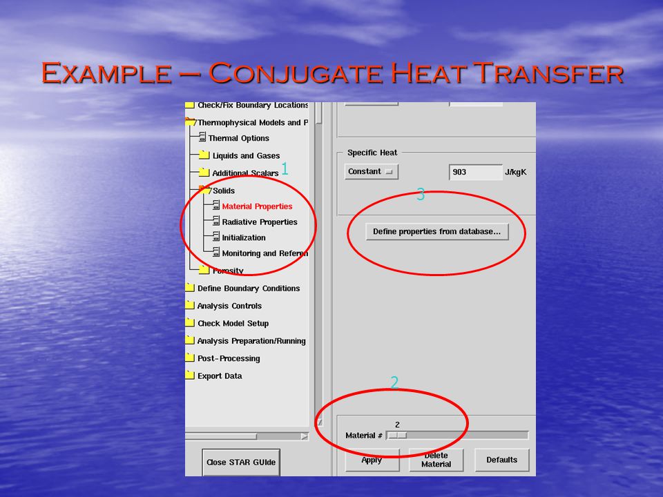
Example – Conjugate Heat Transfer
Heat conduction in a solid and convection in a fluid are considered in conjugate heat transfer. At least, two materials shall be defined as a fluid and a solid in the model, respectively.

44
Example – Conjugate Heat Transfer
.

45
Example – Conjugate Heat Transfer
T = 293 K air g 0.01 m Adiabatic boundary Adiabatic boundary 0.01 m Al T = 294 K

46
Example – Conjugate Heat Transfer
1 3 2
47
Example – Conjugate Heat Transfer
4. Choose a solid material from the table or creat a new one. Do not forget to click apply.

48
Example – Conjugate Heat Transfer
5. Use C> /NEW / Zone to select cells into cset.

49
Example – Conjugate Heat Transfer
6. Click Tools/Cell Tools to set Type 2 Solid to Material 2

50
Example – Conjugate Heat Transfer
7. Use cell list to change cells in cset to the type 2 solid

51
Example – Conjugate Heat Transfer
8. Check if there are two different kinds of cells. Red one is fluid 1. Green one is solid 2.

52
Example – Conjugate Heat Transfer
Go back to STAR Guide. Click Thermal Options. Click Heat Transfer ON. The rest procedures for simulation of natural convection are as same as the previous example.

53
Example – Conjugate Heat Transfer
Iosthermal contours + Velocity vectors

Similar presentations

 Method for Mixed Heat Transfer>")


>")
