1. Computer Aided Thermal Fluid Analysis Lecture 7 Dr. Ming-Jyh Chern ME NTUST

2. Road Map for Today Example of arbitrary couple Example of arbitrary couple Solver for a steady laminar flow problem Solver for a steady laminar flow problem Setup solver step by step Setup solver step by step Simple post-processing – velocity and contour plots Simple post-processing – velocity and contour plots User Guide Chapter 8 User Guide Chapter 8

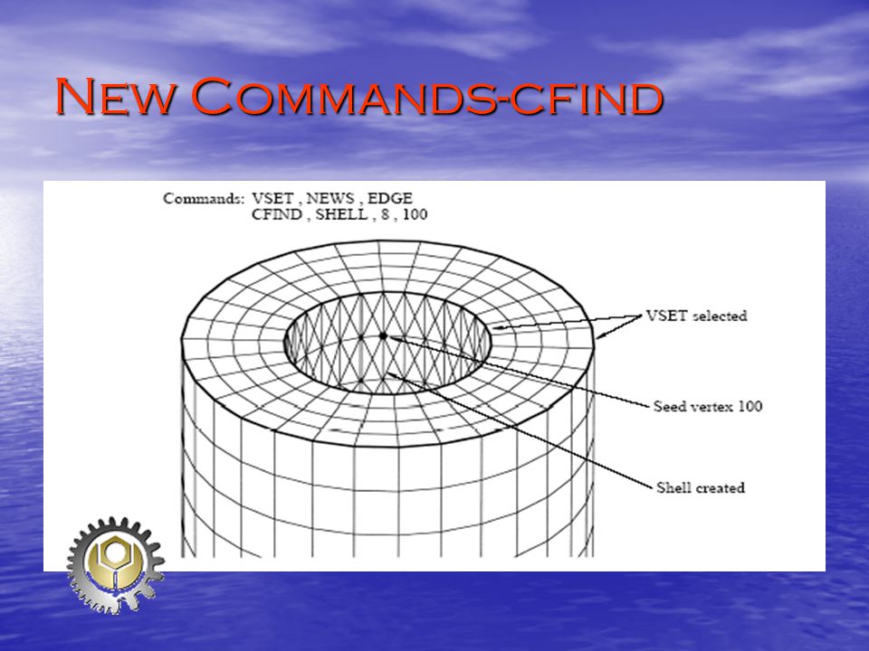
3. New Commands-cfind

6. New Commands-vpro

9. New Commands-crefine

12. Example of Arbitrary Couple

15. Solver for a Steady Laminar Flow Steady flow – Steady flow – Laminar flow – fluid flows without turbulent fluctuations. Laminar flow – fluid flows without turbulent fluctuations. You’d better understand your problem as detail as possible before you regard your problem as a steady laminar flow. You’d better understand your problem as detail as possible before you regard your problem as a steady laminar flow.

16. Before you go to the solver You need to finished tasks of pre- processing: You need to finished tasks of pre- processing: – Mesh setup up – Fluid property and thermofluid model specification – Definition of boundary type and location

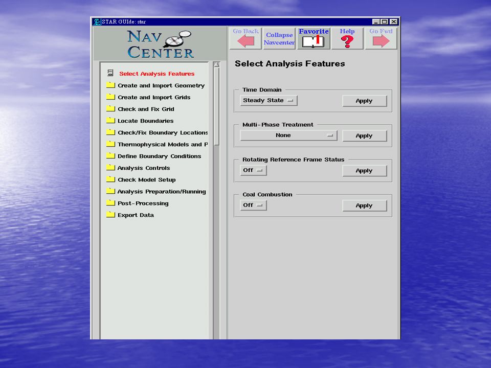
17. Quickest Way to Solve Steady Flow I Step 1 – Select Steady State from the Time domain pop-up menu in the STAR-GUIde Step 1 – Select Steady State from the Time domain pop-up menu in the STAR-GUIde Step 2 – Go to the Solution Controls folder and open the Solution Method panel. Choose Steady State or Pseudo-Transient Step 2 – Go to the Solution Controls folder and open the Solution Method panel. Choose Steady State or Pseudo-Transient

20. Quickest Way to Solve Steady Flow II Step 3 – In the Primary Variables panel, Step 3 – In the Primary Variables panel, Step 4 – Relaxation and Solve Parameters, set up tolerance and iterative number Step 4 – Relaxation and Solve Parameters, set up tolerance and iterative number Step 5 - Choose one of the available Differential Schemes. Step 5 - Choose one of the available Differential Schemes.

24. Quickest Way to Solve Steady Flow III Step 6 – Output control. Monitor Numeric Behavior Step 6 – Output control. Monitor Numeric Behavior Step 7 – Output control. Analysis control Step 7 – Output control. Analysis control Step 8 - Save & Check model setup. Step 8 - Save & Check model setup.

28. Quickest Way to Solve Steady Flow IV Step 9 – Analysis preparation / Running. Set run time control Step 9 – Analysis preparation / Running. Set run time control Step 10 - Analysis preparation / Running. Analysis (Re)start Step 10 - Analysis preparation / Running. Analysis (Re)start

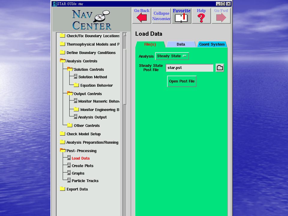
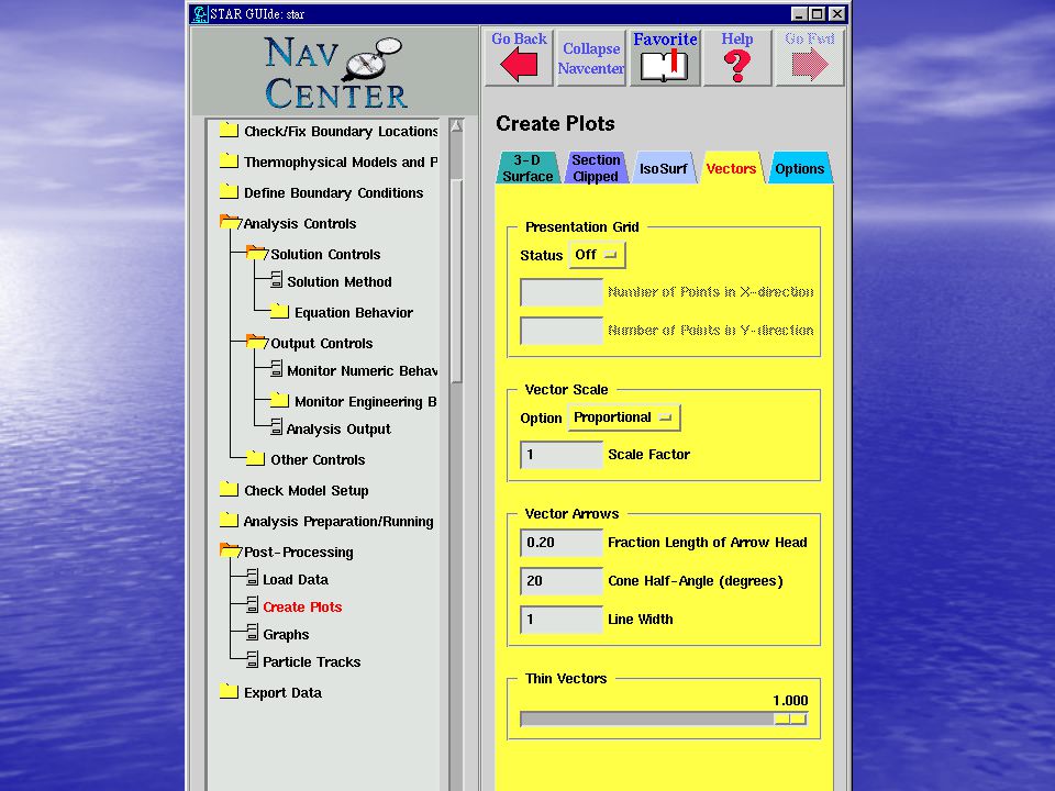
32. PostProcessing Load Data Load Data Create plots Create plots Export data Export data

39. Homework 4 Simulate a 2-D lid-driven cavity flow at Re = 100 and 1,000. Please compare your velocity results with Ghia et al.’s(1982) data along the vertical central line. Simulate a 2-D lid-driven cavity flow at Re = 100 and 1,000. Please compare your velocity results with Ghia et al.’s(1982) data along the vertical central line. Simulate a 2-D uniform flow past a circular cylinder at Re = 40. Predict the length l of the wake behind the circular cylinder of diameter d. Simulate a 2-D uniform flow past a circular cylinder at Re = 40. Predict the length l of the wake behind the circular cylinder of diameter d. Choose one of them. Give velocity and pressure contour plot first. Subsequently, you have to make the required comparison. Choose one of them. Give velocity and pressure contour plot first. Subsequently, you have to make the required comparison. Due date: 15 May, 2006 Due date: 15 May, 2006 Ghia, U., Ghia, K.N., and Shin, C.T. 1982 High-Re solutions for incompressible flow using the Navier-Stokes equations and a multigrid method. Journal of Computational Physics 48, 387-411. Ghia, U., Ghia, K.N., and Shin, C.T. 1982 High-Re solutions for incompressible flow using the Navier-Stokes equations and a multigrid method. Journal of Computational Physics 48, 387-411.

40. Homework 4 – Problem I U L 0.5L Re = UL/ Compare your solution of horizontal velocity component with Ku et al. ’ s along this central vertical line.

41. Homework 4 – Problem I Rey1001,000 1.0001.01.0 0.97660.841230.65928 0.96880.788710.57492 0.96090.737220.51117 0.95310.687170.46604 0.85160.231510.33304 0.73440.003320.18719 0.6172-0.136410.05702 0.5-0.20581-0.06080 0.4531-0.21090-0.10648 0.2813-0.15662-0.27805 0.1719-0.10150-0.38289 0.1016-0.06434-0.2973 0.0703-0.04775-0.2222 0.0625-0.04192-0.20196 0.0547-0.03717-0.18109 0.000 Profile of velocity component u along the central vertical line.

42. Homework 4 – Problem I

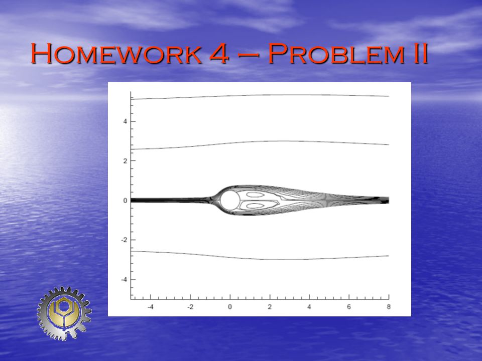
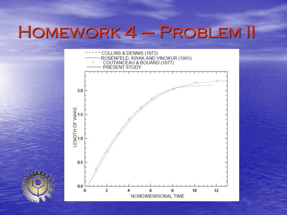
44. Homework 4 – Problem II U D Re = UD/ l Please calculate l /D from the steady solution at Re = 40.

45. Homework 4 – Problem II