1. PhD remote sensing course, 2013 Lund University Understanding Vegetation indices PART 1 Understanding Vegetation indices PART 1 : General Introduction Talk by Hongxiao Jin

2. Light interaction with canopy Transmittance and reflectance PART 1

3. Ground area A a Opaque leaf area a A

4. A Ground area A, N opaque leaves

5. black leaf, a=1 For transparent any LAD leaves absorptivity a Canopy transmittance for horizontal opaque leaf

6. Transmittance model from simple exponential equation. a=0.8 for PAR (or red), a=0.2 for NIR. In comparison with SAIL model.

7. Figure: canopy transmittance from in situ 4-sensor PAR component measurements (Eklundh et al., 2011). PAR (or red) transmittance is much larger than modelled. In Abisko the caopy LAI is ca. 0.8-1.9

8. Simplest RT equation Boundary conditions Solution

9. LAI Horizontal leaves Thin flat leaf

10. Horizontal leaves Can be understood from optical path and cross-section area.

11. Leaf angle distribution probability density function: G(  l ) Random leaves I I 0 i  is the angle between sun beam and leaf normal Cross-section area Average ratio of shadow cast area onto horizontal surface to each single leaf area

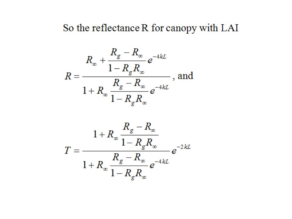
15. Canopy reflectance Boundary conditions

17. Hapke diffusive reflectance theory

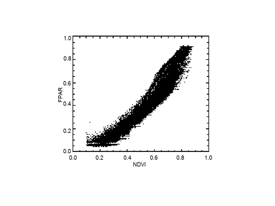
19. Estimate FPAR from measured canopy reflectance Suppose

22. Vegetation indices PART 2

23. The history of VIs NDVI Dr. John Rouse, the Director of the Remote Sensing Center of Texas A&M University where the Great Plains study was conducted with Landsat-1 PhD student Donald Deering and his advisor Dr. Robert Haas With the assistance of a resident mathematician (Dr. John Schell) To “normalize” the effects of the solar zenith angle

24. NDVI is simple, easy to use, by correlating with ground observation. and therefore, NDVI is over-used (abused) Use NDVI for LAI fAPAR fraction of vegetation cover water content preciptation Leaf nitrogen content chlorophyll concentration in leaf Biomass Plant productivity (GPP/NPP) Vegetation stress monitoring Vegetation disturbance Flowering phenology Rats activity Grazing monitoring …

25. https://ecocast.adobeconnect.com/_a954016155/p3dz6o2fuv6/?launcher=false&fcsCont ent=true&pbMode=normal 00:25:39 -00:27:10

26. NDVI~fAPAR Observed direct proportional relationship Attempt to prove it by prof. Knyazikhin The well-known fAPAR product only use this direct proportional relationship as backup algorithm to infer fAPAR from NDVI

30. Figure: RVI has a good linear relationship with total wet biomass (Data point are digitized from Tucker (1979)’s NDVI paper)

31. Vegetation isolines from Huete’s cotton field experiment For l 1 =l 2 =L/2

32. Vegetation isoline modelled from Hapke diffusive reflectance (same as from SAIL model)

37. NDVIEVIEVI2DVIRVIVPILVIAVI CV(±60)0.050.13 0.180.160.240.200.23 NDVIEVIEVI2DVIRVIVPILVIAVI CV(±15)0.010.03 0.040.020.05 Principal plane

38. Perpendicular to principal plane NDVIEVIEVI2DVIRVIVPILVIAVI CV(±60)0.040.080.070.080.120.100.090.10 NDVIEVIEVI2DVIRVIVPILVIAVI CV(±15)0.00 0.01 0.000.01