1. Chapter 6 Demand The demand function gives the optimal amounts of each of the goods as a function of the prices and income faced by the consumer: x 1 (p 1, p 2, m) We now change the arguments in the demand function one by one. ∆x 1 /∆m > 0: good 1 is a normal good ∆x 1 /∆m < 0: inferior (depends on the income level we are talking about: bus, MRT, taxi)

2. Fig. 6.1

3. Fig. 6.2

4. Two ways to look at the same thing (1) At x 1 – x 2 space, connect the demanded bundles as the budget line gets shifted outward. This curve is called the income offer curve (IOC) or income expansion path. (2) At x 1 – m space, connect the optimal x 1 bundles as the income increases while holding all prices fixed. This curve is called the Engel curve.

5. Fig. 6.3

6. Draw a general preference to illustrate the income offer curve and the Engel curve. Perfect substitutes: p 1 p 2 and p 1 = p 2. Perfect complements: IOC (at the corner), Engel (sloped p 1 + p 2 ) Cobb-Douglas: x 1 = am/ p 1 and x 2 = (1- a)m/ p 2 so x 1 /x 2 is constant, thus IOC (line), Engel (sloped p 1 /a))

7. Fig. 6.4

8. Fig. 6.5

9. Fig. 6.6

10. In the above three cases, (∆x 1 / x 1 )/(∆m/m) = 1. They all belong to homothetic preferences. If (x 1, x 2 ) w (y 1, y 2 ), then for all t >0, (tx 1, tx 2 ) w (ty 1, ty 2 ). ( 無異曲線等 比例放大縮小 )

11. If (x 1, x 2 ) is optimal at m, then (tx 1, tx 2 ) is optimal at tm. Suppose not, then (y 1, y 2 ) is feasible at tm and (y 1, y 2 ) s (tx 1, tx 2 ). Then (y 1, y 2 ) w (tx 1, tx 2 ) and it is not the case that (tx 1, tx 2 ) w (y 1, y 2 ). However, (y 1 /t, y 2 /t) is feasible at m, so (x 1, x 2 ) w (y 1 /t, y 2 /t). By homothetic preferences, (tx 1, tx 2 ) w (y 1, y 2 ), a contradiction.

12. Reasonable? (toothpaste) Quasilinear preferences: p 1 = p 2 =1, u(x 1, x 2 ) = √x 1 + x 2 MU 1 = 1/(2 √x 1 ), MU 2 = 1, MU 1 /p 1 = MU 2 /p 2 implies x 1 = ¼ IOC: on the x-axis up to (1/4,0), then becomes vertical Engel: sloped 1 up to (1/4, 1/4), then becomes vertical “zero income effect” only after some point

13. Fig. 6.8

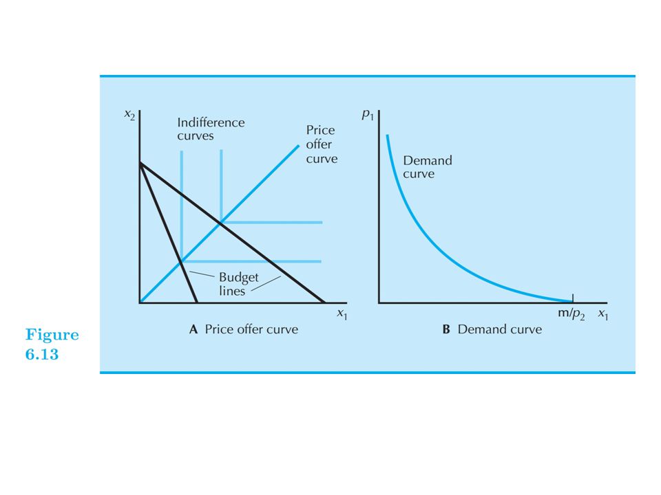
14. ∆x 1 /∆p 1 > 0: good 1 is a Giffen good ∆x 1 /∆p 1 < 0: good 1 is an ordinary good Two ways to look at the same thing (1) At x 1 – x 2 space, connect the demanded bundles as the budget line gets pivoted outward. This curve is called the price offer curve (POC).

15. (2) At x 1 – p 1 space, connect the optimal x 1 bundles as own price increases while holding income and other price fixed. This curve is called the demand curve. Draw a general preference to illustrate the price offer curve and the demand curve.

16. Fig. 6.9

17. Fig. 6.11

18. Perfect substitutes: POC p 1 > p 2 : x 1 = 0, p 1 = p 2 : all budget line, p 1 < p 2 : x 1 = m/ p 1, draw demand curve Perfect complements: POC (at the corner), demand (m/(p 1 +p 2 )) Discrete: good 1 is in discrete amounts and u(x 1, x 2 ) = v(x 1 ) + x 2

19. Fig. 6.12

21. Suppose m is large enough in the relevant range and let x 2 be the amount of money you can spend on all other goods, then you will start to buy the first unit of good 1 when p 1 has decreased to v(0)+m = v(1)+m-p 1, so p 1 has decreased to v(1) – v(0). Similarly, you will start buying the second unit of good 1 when p 1 has further decreased to v(1)+m-p 1 = v(2)+m-2p 1, so p 1 has decreased to v(2) – v(1). (draw) Illustrate the demand curve for the quasilinear case

22. Fig. 6.14

23. ∆x 1 /∆p 2 > 0: good 1 is a substitute for good 2 ∆x 1 /∆ p 2 < 0: good 1 is a complement for good 2 ( 像自己價格的改變 ) The inverse demand function x 1 = x 1 (p 1 ), given p 1, how many x 1 that a consumer wants to buy p 1 = p 1 (x 1 ), given x 1, what price of p 1 would have to be in order for the consumer to choose that level of consumption

24. Fig. 6.15

25. Cobb Douglas x 1 = am/ p 1 vs. p 1 = am/ x 1 Inverse demand has a useful interpretation |MRS 1, 2 | = p 1 / p 2 so p 1 = |MRS 1, 2 | p 2 suppose good 2 is the money to spend on all other goods, so p 2 = 1 and p 1 = |MRS 1,2 | = ∆$/∆ x 1 : how many dollars the individual would be willing to give up to have a little more of 1 (marginal willingness to pay)

26. Demand downward sloping is due to that the marginal willingness to pay decreases as x 1 increases (different from diminishing MRS along an indifference curve).