1. Hypothesis Tests II

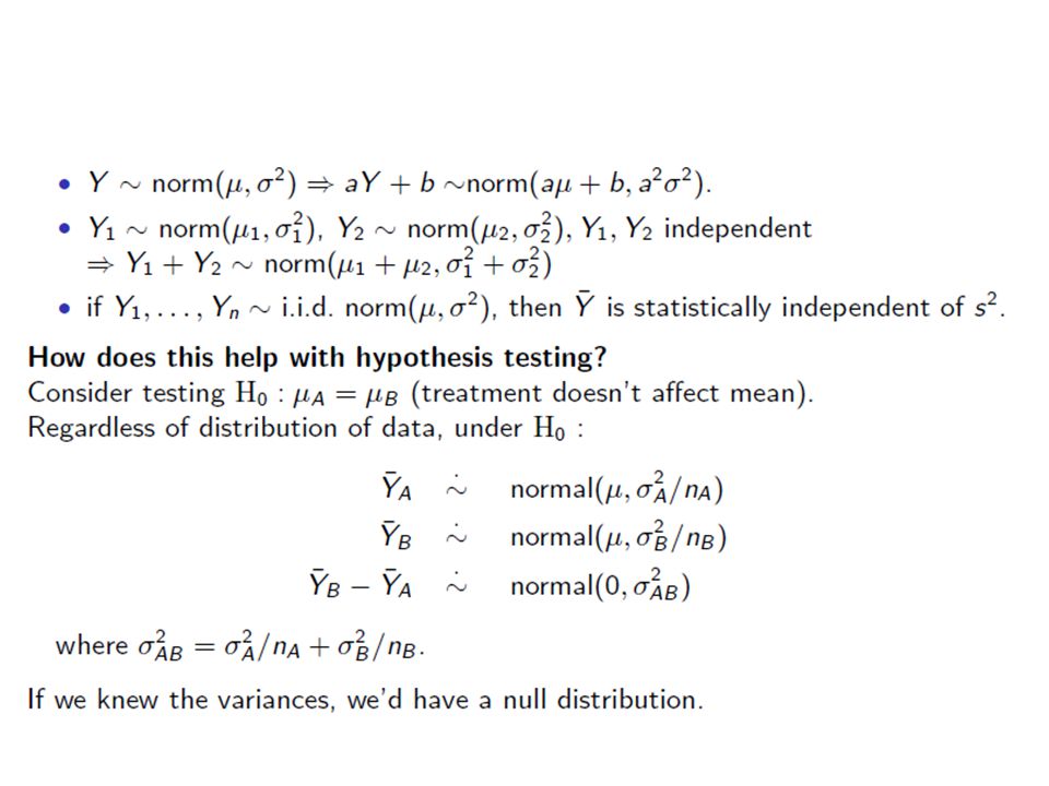
2. The normal distribution

3. Normally distributed data

4. Normally distributed means

6. First, lets consider a more simple problem…

11. z1z1 z2z2

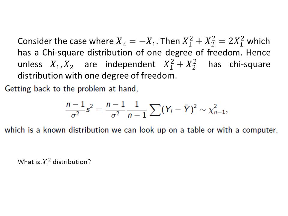
12. z1z1 z2z2 This is how one dimension (degrees of freedom) is lost!

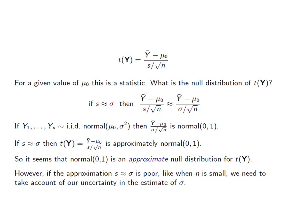
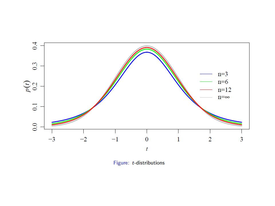
16. The t-distribution

17. That is why we divide by (n-1) in calculating sample s.d.

19. One sample t-test

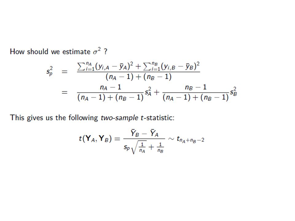
22. Two-sample tests B and A are types of seeds.

24. Numerical Example (wheat again)

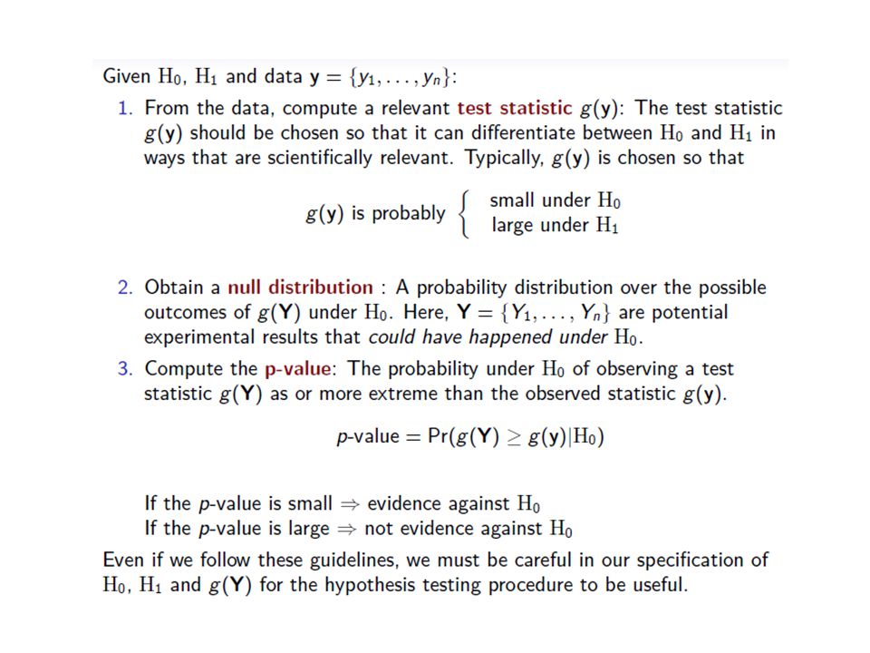
25. Summary: We have so far seen how a good test statistic (null distribution) looks like. The distribution that we have selected is a test book distribution. Could we pick others?

27. Choosing Test Statistic

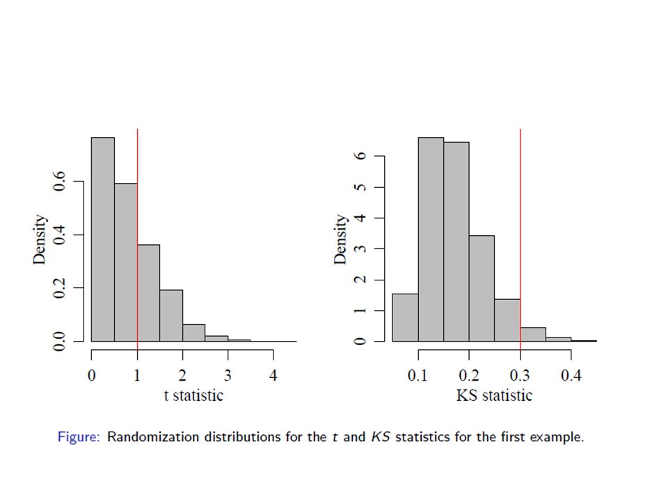
28. The t statistic

29. The Kolmogorov-Smirnov statistic

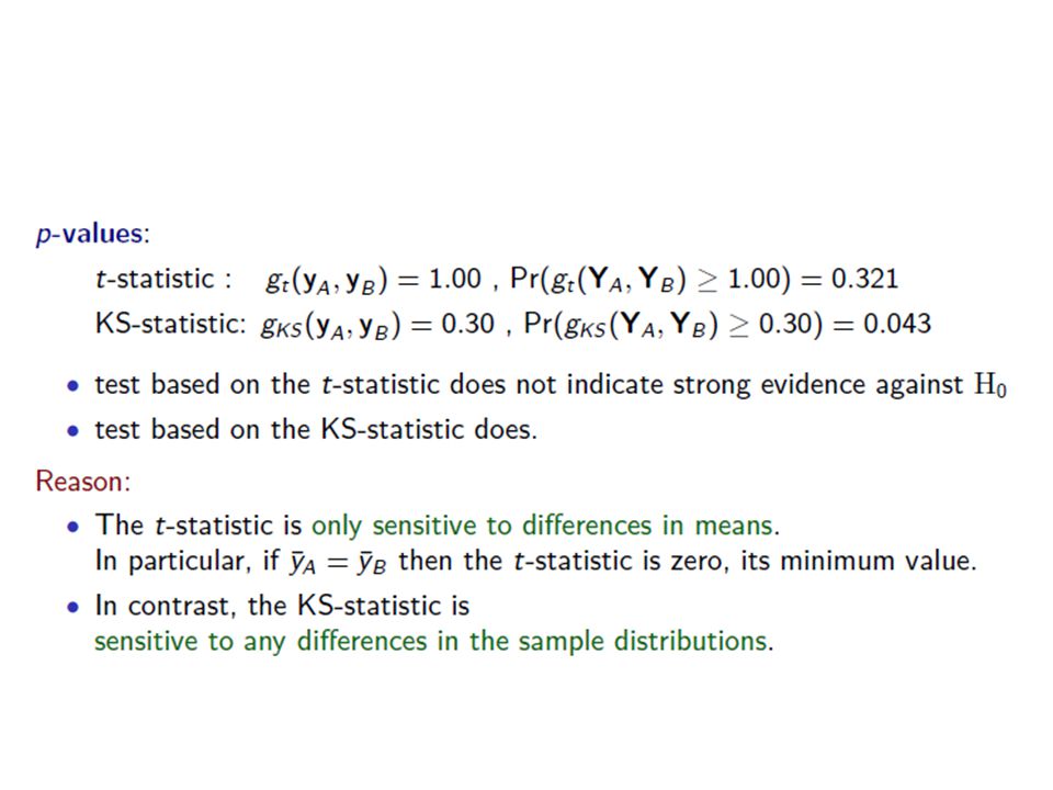
30. Comparing the test statistics

33. Sensitivity to specific alternatives

35. Discussion

36. Or… We need to add in additional assumptions such as equality of the stanadard deviations of the samples.

37. Two-sample tests B and A are types of seeds.

38. Contingency Tables (Cross-Tabs)

39. We use cross-tabulation when: We want to look at relationships among two or three variables. We want a descriptive statistical measure to tell us whether differences among groups are large enough to indicate some sort of relationship among variables.

40. Cross-tabs are not sufficient to: Tell us the strength or actually size of the relationships among two or three variables. Test a hypothesis about the relationship between two or three variables. Tell us the direction of the relationship among two or more variables. Look at relationships between one nominal or ordinal variable and one ratio or interval variable unless the range of possible values for the ratio or interval variable is small. What do you think a table with a large number of ratio values would look like?

41. Because we use tables in these ways, we can set up some decision rules about how to use tables Independent variables should be column variables. If you are not looking at independent and dependent variable relationships, use the variable that can logically be said to influence the other as your column variable. Using this rule, always calculate column percentages rather than row percentages. Use the column percentages to interpret your results.

42. For example, If we were looking at the relationship between gender and income, gender would be the column variable and income would be the row variable. Logically gender can determine income. Income does not determine your gender. If we were looking at the relationship between ethnicity and location of a person’s home, ethnicity would be the column variable. However, if we were looking at the relationship between gender and ethnicity, one does not influence the other. Either variable could be the column variable.

43. Contingency Tables (Cross-Tabs) Marital Status MarriedSingle Gender Male3741 Female5132 How do we measure the relationship?

44. What do we EXPECT if there is no relationship? GenderTotal FemaleMale Result Cured78 Not83 Total8873161

45. ObservedExpected FMFM Cured3741Cured42.635.4 Not5132Not45.437.6 3.18

46. RESULT ● This test statistic has a χ 2 distribution with (2-1)(2-1) = 1 degree of freedom ● The critical value at α =.01 of the χ2 distribution with 1 degree of freedom is 6.63 ● Thus we do not reject the null hypothesis that the two proportions are equal, that the drug is equally effective for female and male patients

47. INTRODUCTION TO ANOVA CASESCORECASESCORE 55 55 55 55 55

48. CASESCORECASESCORE 5+2=75-2=3 5+2=75-2=3 5+2=75-2=3 5+2=75-2=3 5+2=75-2=3

50. The third step is to complete the GLM with addition of error. CASESCORECASESCORE 5+2+2=95-2+0=3 5+2+0=75-2-2=1 5+2-1=65-2+0=3 5+2+0=75-2+1=4 5+2-1=65-2+1=4

52. Standard Setup for ANOVA Sum 93 71 63 74 64

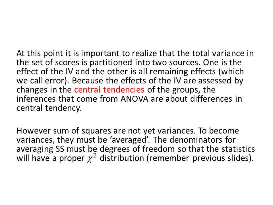
53. Sum of squares for treatment The effect of the IV!!! Sum of squares for treatment The effect of the IV!!! Sum of squares for error Each term is then squared and summed seperately to produce the sum of squares for error and the sum of squares for treatment seperately. The basic partition holds because the cross product terms vanish.

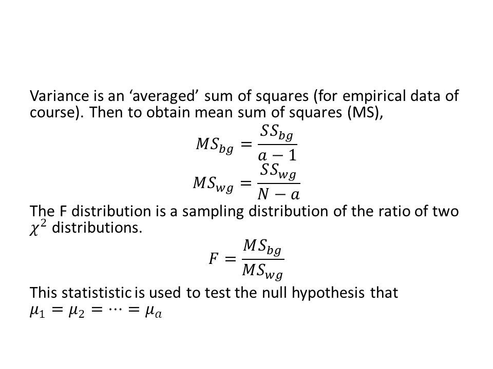
58. Source table for basic ANOVA SourceSSdfMSF Between401 26.67 Within1281.5 Total529