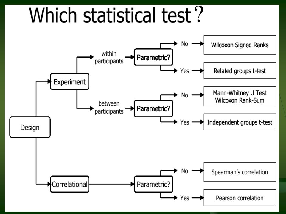
1. NON-PARAMETRIC TEST

2. Statistical tests fall into two categories: (i) Parametric tests (ii) Non-parametric tests

3. The parametric tests make the following assumptions the population is normally distributed; homogeneity of variance If any or all of these assumptions are untrue then the results of the test may be invalid. it is safest to use a non-parametric test.

4. ADVANTAGES OF NON-PARAMETRIC TESTS If the sample size is small there is no alternative If the data is nominal or ordinal These tests are much easier to apply

5. DISADVANTAGES OF NON-PARAMETRIC TESTS i)Discard information by converting to ranks ii)Parametric tests are more powerful iii)Tables of critical values may not be easily available. iv)It is merely for testing of hypothesis and no confidence limits could be calculated.

6. Non-parametric tests Note: When valid, use parametric Note: When valid, use parametric Commonly used Commonly used Wilcoxon signed-rank test Wilcoxon rank-sum test Spearman rank correlation Chi square etc. Useful for non-normal data Useful for non-normal data If possible use some transformation If possible use some transformation If normalization not possible If normalization not possible Note: CI interval -difficult/impossible Note: CI interval -difficult/impossible

7. ?

8. Wilcoxon signed rank test To test difference between paired data To test difference between paired data

9. Patient Hours of sleep DrugPlacebo 16.15.2 27.07.9 38.23.9 47.64.7 56.55.3 68.45.4 76.94.2 86.76.1 97.43.8 105.86.3 EXAMPLE Null Hypothesis: Hours of sleep are the same using placebo & the drug

10. STEP 1 Exclude any differences which are zero Exclude any differences which are zero Ignore their signs Ignore their signs Put the rest of differences in ascending order Put the rest of differences in ascending order Assign them ranks Assign them ranks If any differences are equal, average their ranks If any differences are equal, average their ranks

11. STEP 2 Count up the ranks of +ives as T + Count up the ranks of +ives as T + Count up the ranks of –ives as T - Count up the ranks of –ives as T -

12. STEP 3 If there is no difference between drug (T + ) and placebo (T - ), then T + & T - would be similar If there is no difference between drug (T + ) and placebo (T - ), then T + & T - would be similar If there is a difference If there is a difference one sum would be much smaller and one sum would be much smaller and the other much larger than expected the other much larger than expected The larger sum is denoted as T The larger sum is denoted as T T = larger of T + and T - T = larger of T + and T -

13. STEP 4 Compare the value obtained with the critical values (5%, 2% and 1% ) in table Compare the value obtained with the critical values (5%, 2% and 1% ) in table N is the number of differences that were ranked (not the total number of differences) N is the number of differences that were ranked (not the total number of differences) So the zero differences are excluded So the zero differences are excluded

14. Patient Hours of sleep DifferenceRank Ignoring sign DrugPlacebo 16.15.20.93.5* 27.07.9-0.93.5* 38.23.94.310 47.64.72.97 56.55.31.25 68.45.43.08 76.94.22.76 86.76.10.62 97.43.83.69 105.86.3-0.51 3 rd & 4 th ranks are tied hence averaged; T= larger of T + (50.5) and T - (4.5) Here, calculated value of T= 50.5; tabulated value of T= 47 (at 5%) significant at 5% level indicating that the drug (hypnotic) is more effective than placebo

15. Wilcoxon rank sum test To compare two groups To compare two groups Consists of 3 basic steps Consists of 3 basic steps

16. Non-smokers (n=15) Non-smokers (n=15) Heavy smokers (n=14) Heavy smokers (n=14) Birth wt (Kg) 3.993.793.60*3.733.213.60*4.083.613.833.314.133.263.543.512.71 3.182.842.903.273.853.523.232.763.60*3.753.593.632.382.34 Null Hypothesis: Mean birth weight is same between non-smokers & smokers

17. Step 1 Rank the data of both the groups in ascending order Rank the data of both the groups in ascending order If any values are equal, average their ranks If any values are equal, average their ranks

18. Step 2 Add up the ranks in the group with smaller sample size Add up the ranks in the group with smaller sample size If the two groups are of the same size either one may be picked If the two groups are of the same size either one may be picked T= sum of ranks in the group with smaller sample size T= sum of ranks in the group with smaller sample size

19. Step 3 Compare this sum with the critical ranges given in table Compare this sum with the critical ranges given in table Look up the rows corresponding to the sample sizes of the two groups Look up the rows corresponding to the sample sizes of the two groups A range will be shown for the 5% significance level A range will be shown for the 5% significance level

20. Non-smokers (n=15) Non-smokers (n=15) Heavy smokers (n=14) Heavy smokers (n=14) Birth wt (Kg) Rank Rank 3.99273.187 3.79242.845 3.60*182.906 3.73223.2711 3.2183.8526 3.60*183.5214 4.08283.239 3.61202.764 3.83253.60*18 3.31123.7523 4.13293.5916 3.26103.6321 3.54152.382 3.51132.341 2.713 Sum=272Sum=163 * 17, 18 & 19are tied hence the ranks are averaged Hence caculated value of T = 163; tabulated value of T (14,15) = 151 Mean birth weights are not same for non-smokers & smokers they are significantly different

21. Spearmans Rank Correlation Coefficient based on the ranks of the items rather than actual values. can be used even with the actual values Examples to know the correlation between honesty and wisdom of the boys of a class. It can also be used to find the degree of agreement between the judgements of two examiners or two judges.

22. R (Rank correlation coefficient) = D = Difference between the ranks of two items N = The number of observations. Note: -1 R 1. i) When R = +1 Perfect positive correlation or complete agreement in the same direction ii) When R = -1 Perfect negative correlation or complete agreement in the opposite direction. iii) When R = 0 No Correlation.

23. Computation i. Give ranks to the values of items. Generally the item with the highest value is ranked 1 and then the others are given ranks 2, 3, 4,.... according to their values in the decreasing order. ii. Find the difference D = R 1 - R 2 where R 1 = Rank of x and R 2 = Rank of y Note that ΣD = 0 (always) iii. Calculate D 2 and then find ΣD 2 iv. Apply the formula.

24. If there is a tie between two or more items. Then give the average rank. If m be the number of items of equal rank, the factor 1(m 3 -m)/12 is added to ΣD 2. If there is more than one such case then this factor is added as many times as the number of such cases, then

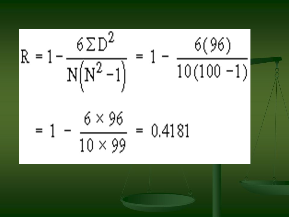
25. Student No. Rank in Maths (R 1 ) Rank in Stats (R 2 ) R 1 - R 2 D (R 1 - R 2 ) 2 D 2 113-24 23124 37439 45500 546 4 669-39 727-525 810824 99 1 1082636 N = 10 Σ D = 0 Σ D 2 = 96