Download presentation
Presentation is loading. Please wait.

1
Algorithms of Google News An Analysis of Google News Personalization Scalable Online Collaborative Filtering 1

2
Overview Data and background Map-Reduce Min-Hash Clustering Probabilistic Latent Semantic Analysis Co-visitation Counts

3
Background Google news is a large multi-user streaming news application The data set has very high churn due to the abundance of new news stories There are too many stories to rely on the users discretion to filter interesting and uninteresting news There are thousands of users with known usage histories in the form of click data Because this is an online system with streaming data (users dont want old news) an offline method will not work.
 an offline method will not work.")
4
Make Decisions for Users The method is called content filtering The goal is to use any data at your disposal about a user and about incoming articles to predict the users interest. More specifically you would need a function that would take a user and an article and generate a prediction for interest (0,1). Then order the list such that articles with a high interest prediction are presented to the user.
. Then order the list such that articles with a high interest prediction are presented to the user..")
5
Available Data We have a limited variety of data, however we have an abundance of a certain type of data from which we can compute metadata about users and news stories. Click Histories Record the stories that a user has clicked on in the past Store this along with all other users click histories in a large table The table consists simply of news articles for columns and users for rows.

6
Map Reduce A large cluster data processing framework Handles all network I/O and fault situations, and is transparent to the application programmer Utilizes Google Filesystem (GFS) a high performance distributed file system. Utilization of map reduce is straightforward, scalable (1000+ machines), and fault tolerant. Mostly just a system programming framework, the parallelization of an algorithm is still up to the application programmer
, and fault tolerant. Mostly just a system programming framework, the parallelization of an algorithm is still up to the application programmer.")
7
Map Reduce In a Nutshell Treat Imperative (like java, c, asm…) functions as pure functions (like lisp, apl, mathematica,Haskel...) Never modify data, simply create new copy of the modified data Functions can take functions, return functions as parameters and output (not really important here) Utilize functional programming basic functions Map and Fold (or Reduce) Mapping is one to one Fold reduces the mapping, by colliding similar objects
 functions as pure functions (like lisp, apl, mathematica,Haskel...) Never modify data, simply create new copy of the modified data Functions can take functions, return functions as parameters and output (not really important here) Utilize functional programming basic functions Map and Fold (or Reduce) Mapping is one to one Fold reduces the mapping, by colliding similar objects")
9
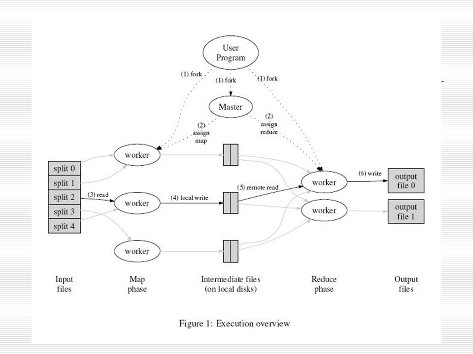
Verbal Explaination of Framework User Program executes the framework. The framework assigns a master computer And partitions the data set over the available workers The workers map the data Once all mapping is complete the workers are reassigned reducing tasks. The result of the reducing tasks are returned to the User Program *All mapping Completes prior to any reducing

10
Map Reduce Ex. (word counts) Map - scan words from documents Map(String key, String value) //key: document name //value: document contents for each word w in value EmitIntermediate(w,1) Reduce – add all words counts together Reduce(String key, Iterator value) //key: a word //value: a list of counts int result = 0 for each v in value: result+= ParseInt(v) Emit(AsString(result))
 Map - scan words from documents Map(String key, String value) //key: document name //value: document contents for each word w in value EmitIntermediate(w,1) Reduce – add all words counts together Reduce(String key, Iterator value) //key: a word //value: a list of counts int result = 0 for each v in value: result+= ParseInt(v) Emit(AsString(result)).")
11
Other Features Some Other Features Locality tuning – try to reduce the data that a node has locally as intermediate data from the map function Fault tolerance – for failed nodes or failed processes Combiner Functions – mini reducer-like function for associative functions. previous example one would likely sum the lists of words found in a document and emitIntermediate() the summed lists instead of every word to save bandwidth.
 the summed lists instead of every word to save bandwidth..")
12
Memory-based Method Makes predictions based on a users past selections For each story generate a vector of users that clicked on the story. Then use a similarity measurement (dot product) in the user-vector space to compute a userss similarity with all other users. Unfortunately this is not scalable O(n^2) to compare all stories with all other stories So we will borrow a previously mentioned comparison technique – Min-wise Hashing
 in the user-vector space to compute a userss similarity with all other users. Unfortunately this is not scalable O(n^2) to compare all stories with all other stories So we will borrow a previously mentioned comparison technique – Min-wise Hashing.")
13
Min-Hash Clustering Clustering algorithm that uses hash intersections to probabilistically cluster similar user data. As we are familiar from previous lecture with min- hashing I will not repeat all aspects of the algorithm As with web page duplicate detection we will utilized the jaccard coefficent as our similarity measurement. S(p,q) = Locality Sensitive Hashing – map data points using several hash functions. The probability of collision is much higher for the min-hashes of similar objects.
 = Locality Sensitive Hashing – map data points using several hash functions. The probability of collision is much higher for the min-hashes of similar objects..")
14
Some tweaks to Min-Hashing Concatenate p hash-keys (generated from p functions) for each user so the probability that any 2 users will agree on a concatenated hash key is S(u i,u j ) p. Concatenation makes the underlying clusters more refined Also increases the average similarity if users in a cluster Repeat the p hashing of users to q clusters in parallel to increase recall Hash each user to q clusters where each cluster is defined by the concatenation of p Min-Hash keys This amounts to a matrix of min-hashes and hash functions Instead of generating all random hash permutations over millions of items, Googe generates a set of independent random seed variables for each min-hash function p. Use the product of p and q(the min-hash value that maps to a specific cluster) to generate an ID for the article. The hash value then severs as a proxy for indexing the random hash permutation. The computed seed and hash values have properties similar to the ideal min-hash values.
 to generate an ID for the article. The hash value then severs as a proxy for indexing the random hash permutation. The computed seed and hash values have properties similar to the ideal min-hash values..")
15
Map-Reduced Min-Hash Clustering Due to the complexity and size of the user history matrices the problem of finding approximate min-hash values is not feasible on a single system As we discussed before the parallel MapReduce framework can be utilized Because Hashing can be performed independently, min-hash is a simple candidate for parallelizing during the map phase Additionally the clustering phase is directly related to the reduction method.

16
Map Read click histories for users in parallel on multiple machines Map inputs to a set of key value pairs computing p x q Min-Hash values for each user Hash each user-id and the random seed corresponding to the hash function Combine the Min-Hash values in q groups of p Min- Hashes (this is the combiner step from map reduce) For each q groups concatenate the MinHash values to obtain the cluster-id The key value pair corresponds to the cluster-id and user-id respectively
 For each q groups concatenate the MinHash values to obtain the cluster-id The key value pair corresponds to the cluster-id and user-id respectively")
17
Partition And Shuffle The key-value pairs are split into partitions(shards) at the end of the map phase Partitions are based on the hash values of the keys Shards are sorted on the keys so that all key value pairs for the same key(cluster-id) appear together
 at the end of the map phase Partitions are based on the hash values of the keys Shards are sorted on the keys so that all key value pairs for the same key(cluster-id) appear together")
18
Reduce For each cluster-id we obtain the list of user-ids that belong to the cluster Then remove clusters with low membership(more of a housekeeping step) In a separate MapReduce process the cluster-user list is transposed to yield a list of clusters for each user to which they belong This is stored as a database and accessed when the user accesses or makes updates to the system The task of re-clustering is done when a new user arrives, or when the model loses accuracy
 In a separate MapReduce process the cluster-user list is transposed to yield a list of clusters for each user to which they belong This is stored as a database and accessed when the user accesses or makes updates to the system The task of re-clustering is done when a new user arrives, or when the model loses accuracy")
19
PLSI- Probabilistic Latent Semantic Indexing A method for collaborative filtering based on probability models generated from user data Models users iI and items jJ as random variable The relationships are learned from the joint probability distributions of users and items as a mixture distribution Hidden variables tT are introduced to capture the relationship The Corresponding ts can be intuited as groups or clusters of users with similar interests

20
Latent Classes * Apologies for the changed variables from the paper Here we see the two way latent class model, p t defines the latent class t, and in PLSI is a probability distribution. p jt and p it are the probability components of the element matrix i,j and are S and U from the paper respectively. The element matrix consists of frequency in click history-story space, where stories are the columns and the rows are the users Formally the model can be written as p(j|i; θ) = p(t | i) p(j | t) The parameter θ represents the conditional probability distribution for p(t | i) and p(j | t) The latent variable t makes the users i and items j conditionally dependent.
 = p(t | i) p(j | t) The parameter θ represents the conditional probability distribution for p(t | i) and p(j | t) The latent variable t makes the users i and items j conditionally dependent..")
21
What are we looking for Learning the co-occurrence model that defines the conditional probabilities associated with θ (namely the p it and p ij ) is the primary computation for PLSI An estimate of these values is obtained by minimizing the empirical logarithmic loss function, (how not bad we can do) L(θ)= -1 / T log(p(j| t; θ)) This function tries to minimize the difference between a story conditioned on the latent class variable t and the users selection of a particular story, for all users and stories. this can of course be inverted to group users too Ex. User 1 chooses story 2 but not 1 log(p(j 2 | i 1 ; θ))0 therefore p(j 2 | t 1 ) 1 log(p(j 1 | i 1 ; θ))<<0 therefore p(j 1 | t 1 ) 0
)0 therefore p(j 2 | t 1 ) 1 log(p(j 1 | i 1 ; θ))<<0 therefore p(j 1 | t 1 ) 0.")
22
How do you get some Zs The method of minimizing the loss function can be obtained with an iterative expectation maximization algorithm EM consists of two steps E step estimates the posterior latent class variables by computing Q latent class variables (generally initialized as a random matrix) Maximization step computes the relevant probability distributions p(j|t) and p(t|i) In this description we can see a relation to gradient or least squares search algorithms The E step is similar to the gradient and estimates the step size While the M step iterates the search
 Maximization step computes the relevant probability distributions p(j|t) and p(t|i) In this description we can see a relation to gradient or least squares search algorithms The E step is similar to the gradient and estimates the step size While the M step iterates the search")
23
Math of EM for Log-Likelihood E-step q*(t;i,j; θ ):= p(t|i,j; θ )=p(j|t)p(t|i) p(j|t) p(t|i) M-Step p(j|t) = q* (t;i,j; θ) ) (for all i) j i q* (t;i,j; θ ) p(j|t) = q* (t;i,j; θ ) (for all j) t j q* (t;i,j; θ )
:= p(t|i,j; θ )=p(j|t)p(t|i) p(j|t) p(t|i) M-Step p(j|t) = q* (t;i,j; θ) ) (for all i) j i q* (t;i,j; θ ) p(j|t) = q* (t;i,j; θ ) (for all j) t j q* (t;i,j; θ )")
24
Map Reducing EM Because this model is clearly too large I=J=10 million, and L=1000 (the number of latent variables) the memory requirement for the probability distributions alone is (I+J)*L*4 = 80 gigs! Unfortunately the method for map reducing EM algorithm is not as straightforward as it was for min-hash. This is mainly because it is iterative and dependent on the previous iteration However if we rearrange the e-step and rewrite the m steps we get the equations on the following page

25
Map Reduced EM Equations Define some new equations N(t,j) = q*(t;i,j; θ) (for all I) - total number of clicks for a story N(t)= j i q*(t;i,j;θ) - total number of clicks for all stories E-step q*(t;i,j; θ):= p(t|i,j; θ)= N(t,j)/N(t) p'(t|i)__ tT p(j|t) p(t|i)
 = q*(t;i,j; θ) (for all I) - total number of clicks for a story N(t)= j i q*(t;i,j;θ) - total number of clicks for all stories E-step q*(t;i,j; θ):= p(t|i,j; θ)= N(t,j)/N(t) p (t|i)__ tT p(j|t) p(t|i)")
26
M-Step p(t|i) = q* (t;i,j; θ ) (for all j) t j (t;i,j; θ ) q*(t:i,j; θ ') can now be computed independently for every (i,j) pair observed in the click logs Map Reduced M Equation
 = q* (t;i,j; θ ) (for all j) t j (t;i,j; θ ) q*(t:i,j; θ ) can now be computed independently for every (i,j) pair observed in the click logs Map Reduced M Equation")
28
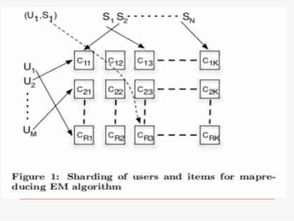
Map Step for Map Reduced EM Using a grid of size R x K mappers users and items can be sharded into r=R,k=K groups as a function of their ids (or randomly) The appropriate click data are sent to the corresponding (r,k) machine where r is the shard that i belongs to and k is the shard for j After computing q*(t;i,j; θ ') the mappers output 3 key value pairs (i,q*) - user shard estimate (j,q*) - item shard estimate (t,q*) -latent class variable estimate
 The appropriate click data are sent to the corresponding (r,k) machine where r is the shard that i belongs to and k is the shard for j After computing q*(t;i,j; θ ) the mappers output 3 key value pairs (i,q*) - user shard estimate (j,q*) - item shard estimate (t,q*) -latent class variable estimate")
29
The reducer shard that receives the key- value pairs for the items j computes N(t,j) (for all t) The reducer shard that receives the key- value pair for I computes p(t|i) And the reducer shard that receives the key-value pair for t computes N(t) The computation in each is the summation of its shards The Map and Reduce steps repeat for each iteration of the EM model until some convergence occurs Map Reduced EM Equations Reducer Step
 (for all t) The reducer shard that receives the key- value pair for I computes p(t|i) And the reducer shard that receives the key-value pair for t computes N(t) The computation in each is the summation of its shards The Map and Reduce steps repeat for each iteration of the EM model until some convergence occurs Map Reduced EM Equations Reducer Step")
30
Co-visitation a simple method of clustering based on the order in which a user clicks on stories Servers track items clicked on by a user within a certain time period The time period decays the value given for a co-visitation count A graph of nodes representing stories and edges representing the time decayed co- visitation instances A newly clicked story and the previous story receives a count when a user views both

31
Putting It Together Sorry for the teaser. The paper that this presentation is on contains detailed information about how this system is implemented, however it is not much of an algorithm (and therefore exceeds the scope of this presentation). also its complicated not in a fun way... like taxes complicated.
. also its complicated not in a fun way... like taxes complicated..")
Similar presentations


>")


