Download presentation
Presentation is loading. Please wait.

1
Advanced Methods and Analysis for the Learning and Social Sciences PSY505 Spring term, 2012 February 1, 2012

2
Today’s Class Diagnostic Metrics

3
Accuracy

4
One of the easiest measures of model goodness is accuracy Also called agreement, when measuring inter- rater reliability # of agreements total number of codes/assessments

5
Accuracy There is general agreement across fields that agreement/accuracy is not a good metric What are some drawbacks of agreement/accuracy?

6
Accuracy Let’s say that Tasha and Uniqua agreed on the classification of 9200 time sequences, out of 10000 actions – For a coding scheme with two codes 92% accuracy Good, right?

7
Non-even assignment to categories Percent accuracy does poorly when there is non- even assignment to categories – Which is almost always the case Imagine an extreme case – Uniqua (correctly) picks category A 92% of the time – Tasha always picks category A Accuracy of 92% But essentially no information
 picks category A 92% of the time – Tasha always picks category A Accuracy of 92% But essentially no information")
8
Kappa

9
(Agreement – Expected Agreement) (1 – Expected Agreement)
 (1 – Expected Agreement)")
10
Kappa Expected agreement computed from a table of the form Model Category 1 Ground Truth Category 1 Count Ground Truth Category 2 Count

11
Cohen’s (1960) Kappa The formula for 2 categories Fleiss’s (1971) Kappa, which is more complex, can be used for 3+ categories – I have an Excel spreadsheet which calculates multi-category Kappa, which I would be happy to share with you
 Kappa The formula for 2 categories Fleiss’s (1971) Kappa, which is more complex, can be used for 3+ categories – I have an Excel spreadsheet which calculates multi-category Kappa, which I would be happy to share with you")
12
Expected agreement Look at the proportion of labels each coder gave to each category To find the number of agreed category A that could be expected by chance, multiply pct(coder1/categoryA)*pct(coder2/categoryA) Do the same thing for categoryB Add these two values together and divide by the total number of labels This is your expected agreement
*pct(coder2/categoryA) Do the same thing for categoryB Add these two values together and divide by the total number of labels This is your expected agreement")
13
Example Detector Off-Task Detector On-Task Ground Truth Off-Task 205 Ground Truth On-Task 1560

14
Example What is the percent agreement? Detector Off-Task Detector On-Task Ground Truth Off-Task 205 Ground Truth On-Task 1560

15
Example What is the percent agreement? 80% Detector Off-Task Detector On-Task Ground Truth Off-Task 205 Ground Truth On-Task 1560

16
Example What is Ground Truth’s expected frequency for on-task? Detector Off-Task Detector On-Task Ground Truth Off-Task 205 Ground Truth On-Task 1560

17
Example What is Ground Truth’s expected frequency for on-task? 75% Detector Off-Task Detector On-Task Ground Truth Off-Task 205 Ground Truth On-Task 1560

18
Example What is Detector’s expected frequency for on-task? Detector Off-Task Detector On-Task Ground Truth Off-Task 205 Ground Truth On-Task 1560

19
Example What is Detector’s expected frequency for on-task? 65% Detector Off-Task Detector On-Task Ground Truth Off-Task 205 Ground Truth On-Task 1560

20
Example What is the expected on-task agreement? Detector Off-Task Detector On-Task Ground Truth Off-Task 205 Ground Truth On-Task 1560

21
Example What is the expected on-task agreement? 0.65*0.75= 0.4875 Detector Off-Task Detector On-Task Ground Truth Off-Task 205 Ground Truth On-Task 1560

22
Example What is the expected on-task agreement? 0.65*0.75= 0.4875 Detector Off-Task Detector On-Task Ground Truth Off-Task 205 Ground Truth On-Task 1560 (48.75)
.")
23
Example What are Ground Truth and Detector’s expected frequencies for off-task behavior? Detector Off-Task Detector On-Task Ground Truth Off-Task 205 Ground Truth On-Task 1560 (48.75)
.")
24
Example What are Ground Truth and Detector’s expected frequencies for off-task behavior? 25% and 35% Detector Off-Task Detector On-Task Ground Truth Off-Task 205 Ground Truth On-Task 1560 (48.75)
.")
25
Example What is the expected off-task agreement? Detector Off-Task Detector On-Task Ground Truth Off-Task 205 Ground Truth On-Task 1560 (48.75)
.")
26
Example What is the expected off-task agreement? 0.25*0.35= 0.0875 Detector Off-Task Detector On-Task Ground Truth Off-Task 205 Ground Truth On-Task 1560 (48.75)
.")
27
Example What is the expected off-task agreement? 0.25*0.35= 0.0875 Detector Off-Task Detector On-Task Ground Truth Off-Task 20 (8.75)5 Ground Truth On-Task 1560 (48.75)
5 Ground Truth On-Task 1560 (48.75).")
28
Example What is the total expected agreement? Detector Off-Task Detector On-Task Ground Truth Off-Task 20 (8.75)5 Ground Truth On-Task 1560 (48.75)
5 Ground Truth On-Task 1560 (48.75).")
29
Example What is the total expected agreement? 0.4875+0.0875 = 0.575 Detector Off-Task Detector On-Task Ground Truth Off-Task 20 (8.75)5 Ground Truth On-Task 1560 (48.75)
5 Ground Truth On-Task 1560 (48.75).")
30
Example What is kappa? Detector Off-Task Detector On-Task Ground Truth Off-Task 20 (8.75)5 Ground Truth On-Task 1560 (48.75)
5 Ground Truth On-Task 1560 (48.75).")
31
Example What is kappa? (0.8 – 0.575) / (1-0.575) 0.225/0.425 0.529 Detector Off-Task Detector On-Task Ground Truth Off-Task 20 (8.75)5 Ground Truth On-Task 1560 (48.75)
 / ( ) 0.225/ Detector Off-Task Detector On-Task Ground Truth Off-Task 20 (8.75)5 Ground Truth On-Task 1560 (48.75).")
32
So is that any good? What is kappa? (0.8 – 0.575) / (1-0.575) 0.225/0.425 0.529 Detector Off-Task Detector On-Task Ground Truth Off-Task 20 (8.75)5 Ground Truth On-Task 1560 (48.75)
 / ( ) 0.225/ Detector Off-Task Detector On-Task Ground Truth Off-Task 20 (8.75)5 Ground Truth On-Task 1560 (48.75).")
33
Interpreting Kappa Kappa = 0 – Agreement is at chance Kappa = 1 – Agreement is perfect Kappa = negative infinity – Agreement is perfectly inverse Kappa > 1 – You messed up somewhere

34
Kappa<0 This means your model is worse than chance Very rare to see unless you’re using cross- validation Seen more commonly if you’re using cross- validation – It means your model is crap

35
0<Kappa<1 What’s a good Kappa? There is no absolute standard

36
0<Kappa<1 For data mined models, – Typically 0.3-0.5 is considered good enough to call the model better than chance and publishable

37
0<Kappa<1 For inter-rater reliability, – 0.8 is usually what ed. psych. reviewers want to see – You can usually make a case that values of Kappa around 0.6 are good enough to be usable for some applications Particularly if there’s a lot of data Or if you’re collecting observations to drive EDM

38
Landis & Koch’s (1977) scale κ Interpretation < 0No agreement 0.0 — 0.20Slight agreement 0.21 — 0.40Fair agreement 0.41 — 0.60Moderate agreement 0.61 — 0.80Substantial agreement 0.81 — 1.00Almost perfect agreement
 scale κ Interpretation < 0No agreement 0.0 — 0.20Slight agreement 0.21 — 0.40Fair agreement 0.41 — 0.60Moderate agreement 0.61 — 0.80Substantial agreement 0.81 — 1.00Almost perfect agreement")
39
Why is there no standard? Because Kappa is scaled by the proportion of each category When one class is much more prevalent – Expected agreement is higher than If classes are evenly balanced

40
Because of this… Comparing Kappa values between two studies, in a principled fashion, is highly difficult A lot of work went into statistical methods for comparing Kappa values in the 1990s No real consensus Informally, you can compare two studies if the proportions of each category are “similar”

41
Kappa What are some advantages of Kappa? What are some disadvantages of Kappa?

42
Kappa Questions? Comments?

43
ROC Receiver-Operating Curve

44
ROC You are predicting something which has two values – True/False – Correct/Incorrect – Gaming the System/not Gaming the System – Infected/Uninfected

45
ROC Your prediction model outputs a probability or other real value How good is your prediction model?

46
Example PREDICTIONTRUTH 0.10 0.71 0.440 0.40 0.81 0.550 0.20 0.10 0.90 0.190 0.511 0.140 0.951 0.30

47
ROC Take any number and use it as a cut-off Some number of predictions (maybe 0) will then be classified as 1’s The rest (maybe 0) will be classified as 0’s
 will then be classified as 1’s The rest (maybe 0) will be classified as 0’s")
48
Threshold = 0.5 PREDICTIONTRUTH 0.10 0.71 0.440 0.40 0.81 0.550 0.20 0.10 0.90 0.190 0.511 0.140 0.951 0.30

49
Threshold = 0.6 PREDICTIONTRUTH 0.10 0.71 0.440 0.40 0.81 0.550 0.20 0.10 0.90 0.190 0.511 0.140 0.951 0.30

50
Four possibilities True positive False positive True negative False negative

51
Which is Which for Threshold = 0.6? PREDICTIONTRUTH 0.10 0.71 0.440 0.40 0.81 0.550 0.20 0.10 0.90 0.190 0.511 0.140 0.951 0.30

52
Which is Which for Threshold = 0.5? PREDICTIONTRUTH 0.10 0.71 0.440 0.40 0.81 0.550 0.20 0.10 0.90 0.190 0.511 0.140 0.951 0.30

53
Which is Which for Threshold = 0.9? PREDICTIONTRUTH 0.10 0.71 0.440 0.40 0.81 0.550 0.20 0.10 0.90 0.190 0.511 0.140 0.951 0.30

54
Which is Which for Threshold = 0.11? PREDICTIONTRUTH 0.10 0.71 0.440 0.40 0.81 0.550 0.20 0.10 0.90 0.190 0.511 0.140 0.951 0.30

55
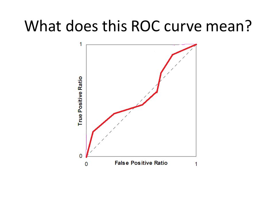
ROC curve X axis = Percent false positives (versus true negatives) – False positives to the right Y axis = Percent true positives (versus false negatives) – True positives going up
 – False positives to the right Y axis = Percent true positives (versus false negatives) – True positives going up")
56
Example

57
What does the pink line represent?

58
What does the dashed line represent?

59
Is this a good model or a bad model?

60
Let’s draw an ROC curve on the whiteboard PREDICTIONTRUTH 0.10 0.71 0.440 0.40 0.81 0.550 0.20 0.10 0.90 0.190 0.511 0.140 0.951 0.30

61
What does this ROC curve mean?

66
ROC curves Questions? Comments?

67
A’ The probability that if the model is given an example from each category, it will accurately identify which is which

68
Let’s compute A’ for this data (at least in part) PREDICTIONTRUTH 0.10 0.71 0.440 0.40 0.81 0.550 0.20 0.10 0.90 0.190 0.511 0.140 0.951 0.30
 PREDICTIONTRUTH")
69
A’ Is mathematically equivalent to the Wilcoxon statistic (Hanley & McNeil, 1982) A really cool result, because it means that you can compute statistical tests for – Whether two A’ values are significantly different Same data set or different data sets! – Whether an A’ value is significantly different than chance

70
Equations

71
Comparing Two Models (ANY two models)
")
72
Comparing Model to Chance 0.5 0

73
Is the previous A’ we computed significantly better than chance?

74
Complication This test assumes independence If you have data for multiple students, you should compute A’ for each student and then average across students (Baker et al., 2008)
")
75
A’ Is also mathematically equivalent to the area under the ROC curve, called AUC (Hanley & McNeil, 1982) The semantics of A’ are easier to understand, but it is often calculated as AUC – Though at this moment, I can’t say I’m sure why – A’ actually seems mathematically easier
 The semantics of A’ are easier to understand, but it is often calculated as AUC – Though at this moment, I can’t say I’m sure why – A’ actually seems mathematically easier")
76
Notes A’ somewhat tricky to compute for 2 categories Not really a good way to compute A’ for 3 or more categories – There are methods, but I’m not thrilled with any; the semantics change somewhat

77
A’ and Kappa What are the relative advantages of A’ and Kappa?

78
A’ and Kappa A’ – more difficult to compute – only works for two categories (without complicated extensions) – meaning is invariant across data sets (A’=0.6 is always better than A’=0.55) – very easy to interpret statistically
 – meaning is invariant across data sets (A’=0.6 is always better than A’=0.55) – very easy to interpret statistically")
79
A’ A’ values are almost always higher than Kappa values Why would that be? In what cases would A’ reflect a better estimate of model goodness than Kappa? In what cases would Kappa reflect a better estimate of model goodness than A’?

80
A’ Questions? Comments?

81
Precision and Recall Precision = TP TP + FP Recall = TP TP + FN

82
What do these mean? Precision = TP TP + FP Recall = TP TP + FN

83
What do these mean? Precision = The probability that a data point classified as true is actually true Recall = The probability that a data point that is actually true is classified as true

84
Precision-Recall Curves Thought by some to be better than ROC curves for cases where distributions are highly skewed between classes No A’-equivalent interpretation and statistical tests known for PRC curves

85
What does this PRC curve mean?

88
ROC versus PRC: Which algorithm is better?

89
Precision and Recall: Comments? Questions?

90
BiC and friends

91
BiC Bayesian Information Criterion (Raftery, 1995) Makes trade-off between goodness of fit and flexibility of fit (number of parameters) Formula for linear regression – BiC’ = n log (1- r 2 ) + p log n n is number of students, p is number of variables
 Makes trade-off between goodness of fit and flexibility of fit (number of parameters) Formula for linear regression – BiC’ = n log (1- r 2 ) + p log n n is number of students, p is number of variables")
92
BiC Values over 0: worse than expected given number of variables Values under 0: better than expected given number of variables Can be used to understand significance of difference between models (Raftery, 1995)
")
93
BiC Said to be statistically equivalent to k-fold cross- validation for optimal k The derivation is… somewhat complex BiC is easier to compute than cross-validation, but different formulas must be used for different modeling frameworks – No BiC formula available for many modeling frameworks

94
AIC Alternative to BiC Stands for – An Information Criterion (Akaike, 1971) – Akaike’s Information Criterion (Akaike, 1974) Makes slightly different trade-off between goodness of fit and flexibility of fit (number of parameters)
 – Akaike’s Information Criterion (Akaike, 1974) Makes slightly different trade-off between goodness of fit and flexibility of fit (number of parameters)")
95
AIC Said to be statistically equivalent to Leave- Out-One-Cross-Validation

96
Which one should you use? “The aim of the Bayesian approach motivating BIC is to identify the models with the highest probabilities of being the true model for the data, assuming that one of the models under consideration is true. The derivation of AIC, on the other hand, explicitly denies the existence of an identifiable true model and instead uses expected prediction of future data as the key criterion of the adequacy of a model.” – Kuha, 2004

97
Which one should you use? “AIC aims at minimising the Kullback-Leibler divergence between the true distribution and the estimate from a candidate model and BIC tries to select a model that maximises the posterior model probability” – Yang, 2005

98
Which one should you use? “There has been a debate between AIC and BIC in the literature, centering on the issue of whether the true model is finite-dimensional or infinite-dimensional. There seems to be a consensus that, for the former case, BIC should be preferred, and AIC should be chosen for the latter.” – Yang, 2005

99
Which one should you use? “Nyardely, Nyardely, Nyoo ” – Moore, 2003

100
Information Criteria Questions? Comments?

101
Diagnostic Metrics Questions? Comments?

102
Next Class Monday, February 6 3pm-5pm AK232 Knowledge Structure (Q-Matrices, POKS, LFA) Barnes, T. (2005) The Q-matrix Method: Mining Student Response Data for Knowledge. Proceedings of the Workshop on Educational Data Mining at the Annual Meeting of the American Association for Artificial Intelligence. Desmarais, M.C., Meshkinfam, P., Gagnon, M. (2006) Learned Student Models with Item to Item Knowledge Structures. User Modeling and User- Adapted Interaction, 16, 5, 403-434. Cen, H., Koedinger, K., Junker, B. (2006) Learning Factors Analysis – A General Method for Cognitive Model Evaluation and Improvement.Proceedings of the International Conference on Intelligent Tutoring Systems, 164-175. Assignments Due: 2. KNOWLEDGE STRUCTURE
 The Q-matrix Method: Mining Student Response Data for Knowledge. Proceedings of the Workshop on Educational Data Mining at the Annual Meeting of the American Association for Artificial Intelligence. Desmarais, M.C., Meshkinfam, P., Gagnon, M. (2006) Learned Student Models with Item to Item Knowledge Structures. User Modeling and User- Adapted Interaction, 16, 5, Cen, H., Koedinger, K., Junker, B. (2006) Learning Factors Analysis – A General Method for Cognitive Model Evaluation and Improvement.Proceedings of the International Conference on Intelligent Tutoring Systems, Assignments Due: 2. KNOWLEDGE STRUCTURE.")
103
The End

Similar presentations


 Curves>")


