Download presentation
Presentation is loading. Please wait.

1
Search by quantum walk and extended hitting time Andris Ambainis, Martins Kokainis University of Latvia

2
Exhaustive search Finite search space. Some elements might be marked. Find a marked element! 1 23 45 6

3
Search with structure Finite search space. Some elements might be marked. Find a marked element! 1 23 45 6 After checking A, it may be easier to check B than C.

4
Example: search on grids N N grid. In one step, we can: – check if vertex marked; – move 1 step;

5
Search by random walk Random walk, following the locality constraints. Stop after finding a marked vertex.

6
Szegedy’2004 Random walk: T steps Quantum walk: O( T) steps
 steps")
7
Szegedy’2004 (fine print) Random walk finds marked element: T steps Quantum walk detects if marked element exists: O( T) steps
 Random walk finds marked element: T steps Quantum walk detects if marked element exists: O( T) steps")
8
Quantum walk detects if marked element exists: O( T) steps
 steps")
9
Quantum walk detects if marked element exists: O( T) steps | start - starting state; No marked element - | start unchanged; Marked elements - | start diverges to an almost orthogonal state | . | not concentrated on marked element

10
Open question Random walk finds marked element: T steps Quantum walk finds marked element: O( T) steps ?
 steps")
11
Krovi, Ozols, Magniez, Roland (previous talk) Quantum algorithm that finds marked element in O( HT + ) steps, HT + - extended hitting time. HT + = HT if there is 1 marked element; HT + can be larger than HT. How large can HT + be?

12
This talk Weak (upper) bound on HT+. Two big gaps between HT+ and HT.
 bound on HT+. Two big gaps between HT+ and HT.")
13
DEFINITIONS

14
Markov chains 1 3 4 2/3 1/3 2 2/3

15
Classical hitting time

16
Matrix form Eigenvalues – real. 1 = 1, eigenvector – stationary distribution. 1 > 2 ... n. Spectral gap: 1- 2. probability of transition i j

17
UPPER BOUND ON HT +

18
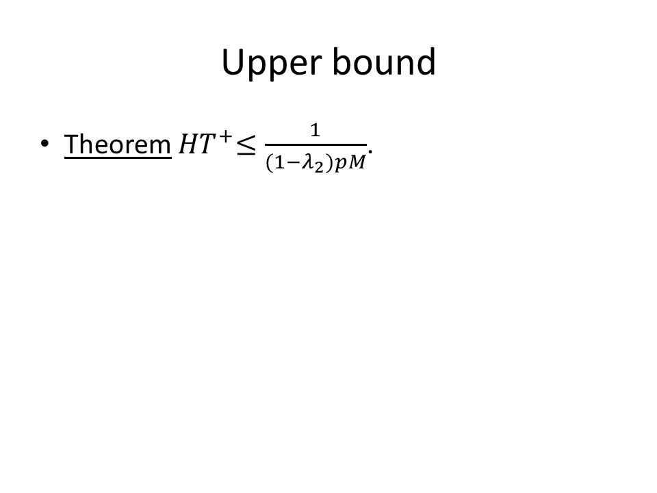
Upper bound

20
1 - 2

21
Corollary

22
How strong is this result?

23
Unstructured search (Grover, 1996) 1 23 45 6
")
24
Grover’s algorithm Query Q: check if an element marked; Diffusion D: – | start | start ; – | -| , | | start . Repeat D, Q, D, Q,..., D, Q.

25
Diffusion Diffusion D: – | start | start ; – | -| , | | start . Markov chain: – |v 1 |v 1 ; – |v i i |v i , i 1- . Can implement diffusion with O(1/ ) steps of Markov chain.
 steps of Markov chain..")
26
Summary KMRO algorithm: – at least as good as Magniez-Nayak-Roland-Santha; – finds 1 marked element optimally. More general description when KMRO works well?

27
GAPS BETWEEN HT+ AND HT

28
Example 1 Stationary distribution: π x =1/3 for all x. M = {1, 2}. HT 10/9. HT+ 1/(4 ). 1 2 3 0.9 0.1 0.9 1- 0.1-
 1- 0.1- .")
29
Example 1 If =0, two eigenvectors with i = 1. If 0, 2 1. Large contribution to HT +, causing HT + . 1 2 3 0.9 0.1 0.9 1- 0.1-

30
Gap between HT and HT+, for a natural search space?

31
2D grid N N grid. Spectral gap: (1/N). Possible: HT + N HT.
. Possible: HT + N HT.")
32
2D grid: example 1 N N grid. HT = (1). HT + = (N). (1) fraction of vertices marked. Classical search easy – no need for quantum.
 fraction of vertices marked. Classical search easy – no need for quantum..")
33
2D grid: example 2 Gap persists, unless the number of marked vertices small.

34
marked unmarked

35
2D grid: example 2 Outside: divide into k k squares, mark corners. Inside: divide into (2k) (2k) squares, mark corners. Regular pattern, with different densities outside and inside.
 (2k) squares, mark corners. Regular pattern, with different densities outside and inside..")
36
Classical hitting time Lower bound: hitting time with 1 marked vertex in each (2k) (2k) square. 1 of 4k 2 vertices marked.

37
Extended hitting time Calculation, using eigenvectors of the grid. HT + = (N), for any density of marked vertices.
, for any density of marked vertices..")
38
KMRO algorithm Result: uniform superposition over marked vertices.

39
KMRO algorithm Pr=1/2 Pr=4/5

40
Marking more elements may increase HT + HT + = (1)HT + = (N)
HT + = (N)")
41
What else can we try?

42
A, Bačkurs, et al., TQC’2013. 2D grid, 1 marked vertex. Standard quantum walk. After O( N log N) steps, state orthogonal to | start . Measurement: Pr[marked] = o(1); Pr[distance N from marked] const.
 steps, state orthogonal to | start . Measurement: Pr[marked] = o(1); Pr[distance N from marked] const..")
43
Idea 1 Does final state | final have large probability on vertices that are close to marked? If true - measure| final , obtain v, search the neighbourhood of v classically.

44
Idea 2 If HT = T, classical walk P hits a marked vertex in O(T) steps, with probability 1- . G’ – neighbourhood of the starting vertex where P stays during O(T) steps. Quantum walk on G’ instead of the full space?
 steps. Quantum walk on G’ instead of the full space .")
45
Conclusions Upper bound for HT +, via spectral gap. KMRO algorithm at least as good as Magniez- Nayak-Roland-Santha. Two examples of gaps between HT + and HT. Optimal quantum algorithm should not be producing the uniform superposition of marked vertices!

Similar presentations
 Joint work with Andris Ambainis (IAS / U. Latvia)>")


 of Quantum Lower Bounds by Polynomials Scott Aaronson UC Berkeley.>")


 Joint work with Andris Ambainis (U. Latvia)>")
 August 14, 2003.>")

, Julia Kempe (Tel Aviv), Or Sattath (Hebrew U.) arXiv:0911.1696.>")


 Brief review of discrete time finite Markov Chain Hidden Markov Model Examples of HMM in Bioinformatics Estimations Basic.>")

 2. Jieping Ye, (Arizona.>")

>")

