Download presentation
Presentation is loading. Please wait.

1
CE 3354 ENGINEERING HYDROLOGY Lecture 6: Probability Estimation Modeling

2
OUTLINE Probability estimation modeling – background Probability plots Plotting positions

3
WHAT IS PROBABILITY ESTIMATION? Use of various techniques to model the behavior of observed data Estimation of the magnitude of some phenomenon (e.g. discharge) associated with a given probability of exceedance Approximate (graphical) methods Mathematical/statistical methods (distribution functions)
 associated with a given probability of exceedance Approximate (graphical) methods Mathematical/statistical methods (distribution functions).")
4
FREQUENCY ANALYSIS Frequency analysis assumes unchanging behavior (stationarity) over time. The time interval is assumed to be long enough so that the concept of “frequency” has meaning (but is NOT periodic). “Long enough” is relative. What is “long enough” for a “frequent” event is not necessarily so for an “infrequent” event. These are the assumptions for analysis only.
. Long enough is relative. What is long enough for a frequent event is not necessarily so for an infrequent event. These are the assumptions for analysis only..")
5
T-YEAR EVENTS The T-year event concept is a way of expressing the probability of observing an event of some specified magnitude or smaller (larger) in one sampling period (one year). Also called the Annual Recurrence Interval (ARI) The formal definition is: The T-year event is an event of magnitude (value) over a long time-averaging period, whose average arrival time between events of such magnitude is T-years (assuming stationarity). The Annual Exceedence Probability (AEP) is a related concept
 The formal definition is: The T-year event is an event of magnitude (value) over a long time-averaging period, whose average arrival time between events of such magnitude is T-years (assuming stationarity). The Annual Exceedence Probability (AEP) is a related concept.")
6
NOTATION P[Q>X] = y Q>X=P[y] We read these statements as “The probability that Q will assume a value greater than X is equal to y”, and “Q is exceeded only associated with the probability of y”
![NOTATION P[Q>X] = y Q>X=P[y] We read these statements as The probability that Q will assume a value greater than X is equal to y , and Q is exceeded only associated with the probability of y](http://images.slideplayer.com/31/9761283/slides/slide_6.jpg "NOTATION P[Q>X] = y Q>X=P[y] We read these statements as The probability that Q will assume a value greater than X is equal to y , and Q is exceeded only associated with the probability of y")
7
FLOOD FREQUENCY CURVE Probability of observing 20,000 cfs or greater in any year is 50% (0.5) (2-year). Exceedance Non-exceedance

8
FLOOD FREQUENCY CURVE Probability of observing 150,000 cfs or greater in any year is ??

9
PROBABILITY MODELS The probability in a single sampling interval is useful in its own sense, but we are often interested in the probability of occurrence (failure?) over many sampling periods. If we assume that the individual sampling interval events are independent, identically distributed then we approximate the requirements of a Bernoulli process.

10
PROBABILITY MODELS As a simple example, assume the probability that we will observe a cumulative daily rainfall depth equal to or greater than that of Tropical Storm Allison in a year is 0.10 (Ten percent). What is the chance we would observe one or more TS Allison’s in a three-year sequence?

11
PROBABILITY MODELS For a small problem we can enumerate all possible outcomes. There are eight configurations we need to consider:

12
PROBABILITY MODELS So if we are concerned with one storm in the next three years the probability of that outcome is 0.243 outcomes 2,3,4; probabilities of mutually exclusive events add. The probability of three “good” years is 0.729. The probability of the “good” outcomes decreases as the number of sampling intervals are increased.

13
PROBABILITY MODELS The probability of the “good” outcomes decreases as the number of sampling intervals are increased. So over the next 10 years, the chance of NO STORM is (.9) 10 = 0.348. Over the next 20 years, the chance of NO STORM is (.9) 20 = 0.121. Over the next 50 years, the chance of NO STORM is (.9) 50 = 0.005 (almost assured a storm).
 10 = Over the next 20 years, the chance of NO STORM is (.9) 20 = Over the next 50 years, the chance of NO STORM is (.9) 50 = (almost assured a storm)..")
14
PROBABILITY MODELS

15
USING THE MODELS Once we have probabilities we can evaluate risk. Insurance companies use these principles to determine your premiums. In the case of insurance one can usually estimate the dollar value of a payout – say one million dollars. Then the actuary calculates the probability of actually having to make the payout in any single year, say 10%. The product of the payout and the probability is called the expected loss. The insurance company would then charge at least enough in premiums to cover their expected loss.

16
USING THE MODELS They then determine how many identical, independent risks they have to cover to make profit. The basic concept behind the flood insurance program, if enough people are in the risk base, the probability of all of them having a simultaneous loss is very small, so the losses can be covered plus some profit. If we use the above table (let the Years now represent different customers), the probability of having to make one or more payouts is 0.271.
, the probability of having to make one or more payouts is")
17
USING THE MODELS If we use the above table, the probability of having to make one or more payouts is 0.271.

18
USING THE MODELS So the insurance company’s expected loss is $271,000. If they charge each customer $100,000 for a $1million dollar policy, they have a 70% chance of collecting $29,000 for doing absolutely nothing. Now there is a chance they will have to make three payouts, but it is small – and because insurance companies never lose, they would either charge enough premiums to assure they don’t lose, increase the customer base, and/or misstate that actual risk.

19
DATA NEEDS FOR PROB. ESTIMATES 1. Long record of the variable of interest at location of interest 2. Long record of the variable near the location of interest 3. Short record of the variable at location of interest 4. Short record of the variable near location of interest 5. No records near location of interest

20
ANALYSIS RESULTS Frequency analysis is used to produce estimates of T-year discharges for regulatory or actual flood plain delineation. T-year; 7-day discharges for water supply, waste load, and pollution severity determination. (Other averaging intervals are also used) T-year depth-duration-frequency or intensity-duration-frequency for design storms (storms to be put into a rainfall-runoff model to estimate storm caused peak discharges, etc.).
 T-year depth-duration-frequency or intensity-duration-frequency for design storms (storms to be put into a rainfall-runoff model to estimate storm caused peak discharges, etc.)..")
21
ANALYSIS RESULTS Data are “fit” to a distribution; the distribution is then used to extrapolate behavior Error function (like a key on a calculator e.g. log(), ln(), etc.) AEP Distribution Parameters Magnitude Module 3
, ln(), etc.) AEP Distribution Parameters Magnitude Module 3.")
22
DISTRIBUTIONS Normal Density Cumulative Normal Distribution

23
DISTRIBUTIONS Gamma Density Cumulative Gamma Distribution

24
DISTRIBUTIONS Extreme Value (Gumbel) Density Cumulative Gumbel Distribution
 Density Cumulative Gumbel Distribution")
25
PLOTTING POSITIONS

26
A plotting position formula estimates the probability value associated with specific observations of a stochastic sample set, based solely on their respective positions within the ranked (ordered) sample set. i is the rank number of an observation in the ordered set, n is the number of observations in the sample set Bulletin 17B

27
PLOTTING POSITION FORMULAS Values assigned by a plotting position formula are solely based on set size and observation position The magnitude of the observation itself has no bearing on the position assigned it other than to generate its position in the sorted series (i.e. its rank) Weibull - In common use; Bulletin 17B Cunnane – General use Blom - Normal Distribution Optimal Gringorten - Gumbel Distribution Optimal
 Weibull - In common use; Bulletin 17B Cunnane – General use Blom - Normal Distribution Optimal Gringorten - Gumbel Distribution Optimal.")
28
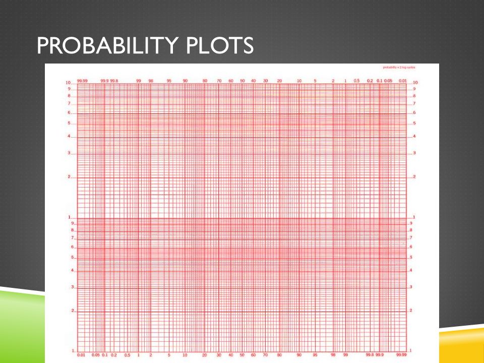
PROBABILITY PLOTS

30
PLOTTING POSITION STEPS 1. Rank data from small to large magnitude. 1. This ordering is non-exceedence 2. reverse order is exceedence 2. compute the plotting position by selected formula. 1. p is the “position” or relative frequency. 3. plot the observation on probability paper 1. some graphics packages have probability scales

31
BEARGRASS CREEK EXAMPLE Examine concepts using annual peak discharge values for Beargrass Creek Data are on class server

32
NEXT TIME Probability estimation modeling (continued) Bulletin 17B
 Bulletin 17B")
Similar presentations
>")


 NERC August 2009.>")
 Frequency Analysis and Probability Plotting.>")


 ISL 2004 RiskCity Introduction to Frequency Analysis of hazardous events.>")

 Precipitation ERS 482/682 Small Watershed Hydrology.>")


