1. Emergence of Complexity in economics Sorin Solomon, Racah Institute of Physics HUJ Israel Scientific Director of Complex Multi-Agent Systems Division, ISI Turin and of the Lagrange Interdisciplinary Laboratory for Excellence In Complexity Coordinator of EU General Integration Action in Complexity Science Chair of the EU Expert Committee for Complexity Science MORE IS DIFFERENT (Anderson 72) (more is more than more) Complex “Macroscopic” properties are often the collective effect of simple interactions between many elementary “microscopic” components MICRO - Investors, individual capital,shares INTER - sell/buy orders, gain/loss MACRO - social wealth distribution, market fluctuations (cycles, crashes, booms, stabilization by noise)

2. 1)I am grateful that our work was not mentioned and thus we were kept out of the dispute. Yet it probably would have weighted in the judgment the physicist-economist cooperation that I had with one leaders of financial economics (Haim Levy) since 1993. Our model have been addressed and/or further developed in papers and PhD’s by three economist groups (Lux +E.Z., F; Chiarella-He; Botazzi-Anufriev). And it concretized in a book that some criticized but other prized… Start from the econo physics critique

3. HARRY M. MARKOWITZ, Nobel Laureate in Economics “Levy, Solomon and Levy's Microscopic Simulation of Financial Markets points us towards the future of financial economics ”

4. 2) In the issue of the power laws: the point is not just to fit by statistical correlations analysis some data to some stylized facts. the point is to understand the causal connection between the behavior at the "microscopic“, individual scale and the emergent phenomena at the "macroscopic“, collective scale. To bridge this scales gap, scaling (not necessaryly criticality) is a natural tool

5. 2) There were the financial economists that limited their attention to stylized facts instead of precise predictions that can be submitted to the Popperian validation. Based on our model, we made precise theoretical predictions connecting measurables that never occurred to economists to compare and then confirmed them a posteriori by empirical measurements. Forbes 400 richest by rank 400 Exponent of Probability of “no significant fluctuation” after time t Pareto-Zipf Exponent in the same economy Pioneers on a new continent: on physics and economics S Solomon and M Levy Quantitative Finance 3, No 1, 2003

6. 3) The physicists did not just bring inappropriate new models they corrected the inappropriate treatment of traditional models that the economists used for a long time. E.g. a model ( the logistic growth ) introduced by the economist Malthus (+Verhuulst) and used continuously and intensively in the last 200 years has been continuously mistreated and thus solutions to long-lived important puzzles were systematically missed by economists until our work. As described below:….

7. A+B-> A+B+B proliferation B->.   death B+B-> B   competition (radius R) almost all the social phenomena, …. obey the logistic growth. “ Social dynamics and quantifying of social forces ” E. W. Montroll I would urge that people be introduced to the logistic equation early in their education… Not only in research but also in the everyday world of politics and economics … Lord Robert May b. = ( a -  )  b –  b 2 (assume 0 dim!!!) Simplest Model: A= gain opportunities, B = capital WELL KNOWN Logistic Equation (Malthus, Verhulst, Lotka, Volterra, Eigen) (no diffusion)

8. A Diffusion of A at rate D a

9. A

10. A

11. A

12. B Diffusion of B at rate D b

13. B

14. B

15. B

16. B A A+B  A+B+B; Birth of new B at rate

17. A B

18. ABAB

19. AB A+B  A+B+B; Birth of new B at rate

20. AB B A+B  A+B+B; Birth of new B at rate

21. ABB A+B  A+B+B; Birth of new B at rate

22. ABB BB A+B  A+B+B; Birth of new B at rate

23. ABB BB A+B  A+B+B; Birth of new B at rate

24. B Another Example A

25. A+B  A+B+B; Birth of new B at rate Another Example A B

26. A+B  A+B+B; Birth of new B at rate Another Example A B

27. A+B  A+B+B; Birth of new B at rate Another Example A AA A B

28. A+B  A+B+B; Birth of new B at rate Another Example A BBBBBB

29. A+B  A+B+B; Birth of new B at rate Another Example A BBB

30. B B B  Death of B at rate 

31. B B B 

32. B B B 

33. B B 

34. Instead: emergence of singular spatio-temporal localized collective patterns with adaptive self-serving behavior => resilience and sustainability even for << 0 !!! prediction: Time Differential Equations continuum  a   << 0 prediction ) Multi-Agent stochastic  a    prediction is ALWAYS wrong in dim >0 The b. = ( a  -  )  b -  b 2 - D b Δb

35. Diff Eq prediction: Time Differential Equations continuum  a   << 0 approx ) Multi-Agent stochastic  a    prediction b. = ( a -  )  b –  b 2 Polish GDP Growth rate after liberalization

36. 5) the capacity of the model to not only organize the stylized facts but to actually predict and explain an enormous amount of data is astonishing..

37. Spatial Correlation of Number of enterprises per capita 98-04 Km The emergence and expansion of the localized adaptive patterns 89 90 91 92 93 94 2004

38. fractal space distribution Prediction of campaign success (15/17) Goldenberg Air-view of a sub-urban neighborhood; crosses on the roofs indicate air-conditioner purchase

39. - Microscopic seeds and Macroscopic Oases MICRO –individual plants INTER –growth, water fixation, MACRO – bushes, vegetation patches N.M. Shnerb, P. Sarah, H. Lavee, and S. Solomon Reactive glass and vegetation patterns Phys. Rev. Lett. 90, 38101 (2003) Mediterranean; uniform Semi-arid; patchy Desert; uniform

40. Technical explanations

41. and Branching Random Walk Theorems (2002) that : - In all dimensions d:  D a > 1-P d always suffices P d = Polya ’ s constant ; P 2 = 1 -On a large enough 2 dimensional surface, the total B population always grows! No matter how fast the death rate , how low the A density, how small the proliferation rate The Importance of Being Discrete; Life Always Wins on the Surface One can prove rigorously by RG

43. First round of intuitions on the effect

44. A one –dimensional simple example continuum prediction A 1 2 3 4 5 6 7 8 9 10 11 12 13 14 B level a =2/14 = 1  1/2 A level

45. A 1 2 3 4 5 6 7 8 9 10 11 12 13 14 B level 2/14 ×× 1 -1/2 = -5/14 A level A one –dimensional simple example continuum prediction a --  ×× t (1-5/14) t continuum prediction

46. b 4 (t+1) = (1 + 1 ×  –   ) b 4 (t) A A 1 2 3 4 5 6 7 8 9 10 11 12 13 14 b 13 (t+1) = (1  + 0 × –   ) b 13 (t) B level A one –dimensional simple example discrete prediction t (1-5/14) t continuum prediction

47. AA 1 2 3 4 5 6 7 8 9 10 11 12 13 14 t (9/14) t Initial exponential decay B level continuum prediction A one –dimensional simple example discrete prediction (3/2) (½)(½) (½)

48. AA 1 2 3 4 5 6 7 8 9 10 11 12 13 14 t (9/14) t (3/2) t B level continuum prediction A one –dimensional simple example discrete prediction (3/2) 2 (½)2(½)2 (½) 2

49. AA 1 2 3 4 5 6 7 8 9 10 11 12 13 14 t (9/14) t (3/2) t growth B level continuum prediction A one –dimensional simple example discrete prediction (3/2) 3 (½)3(½)3 (½) 3

50. AA 1 2 3 4 5 6 7 8 9 10 11 12 13 14 t (9/14) t (3/2) t growth continuum prediction A one –dimensional simple example discrete prediction (3/2) 4 (½)4(½)4 (½) 4

51. AA 1 2 3 4 5 6 7 8 9 10 11 12 13 14 t (3/2) t growth (9/14) t continuum prediction A one –dimensional simple example discrete prediction (3/2) 5 (½)5(½)5 (½) 5

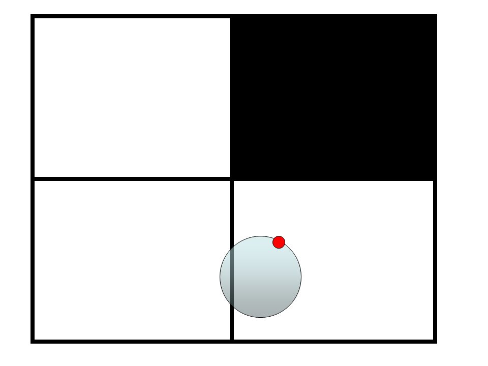
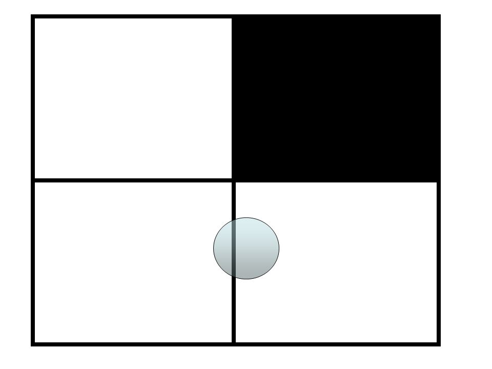
52. A 1 2 3 4 5 6 7 8 9 10 11 12 13 14 The Role of DIFFUSION The Emergence of Adaptive B islands Take just one A in all the lattice:

53. A

54. A

55. A B diffusion

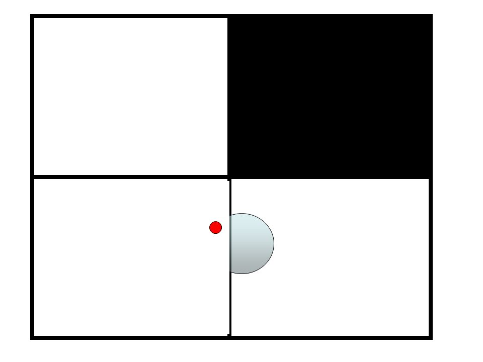
56. A

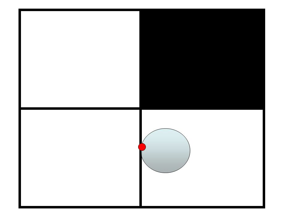
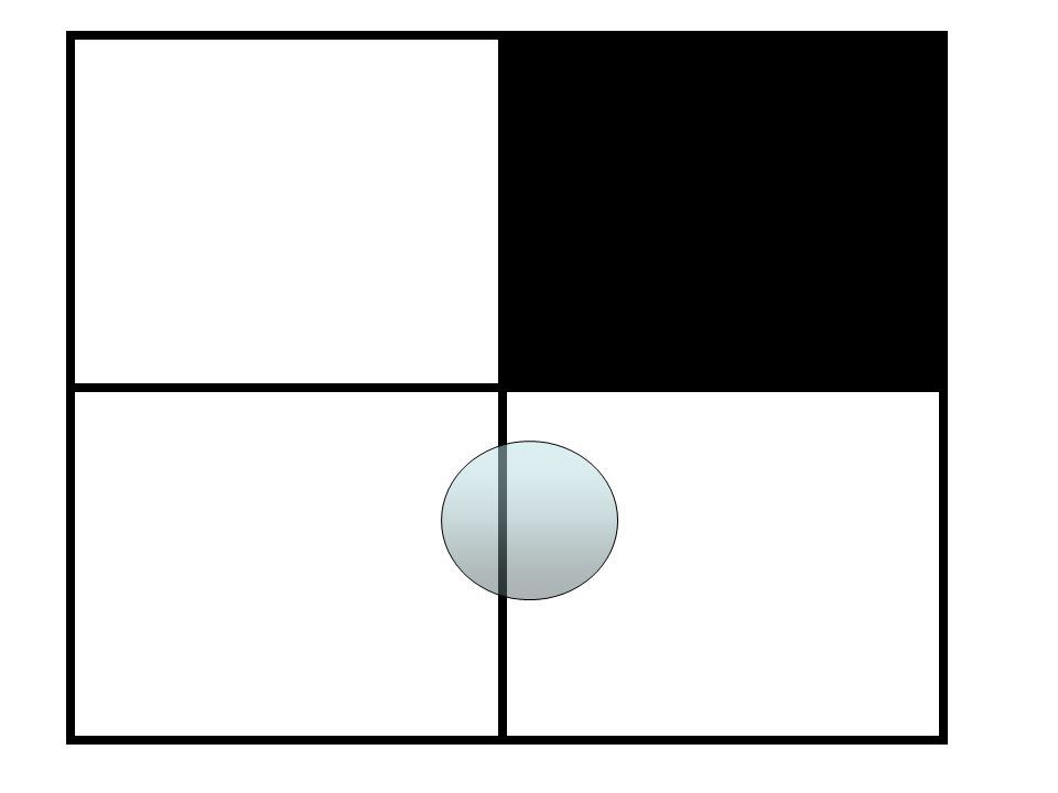
57. A Growth stops when A jumps to a neighboring site

58. AA

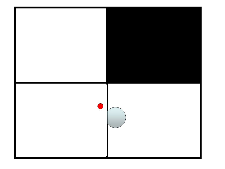
59. A Growth will start on the New A site B population on the old A site will decrease

60. A

61. A

62. A AA

63. A AA

64. A AA

65. A AA B diffusion

66. A AA

67. A AA

68. A AA

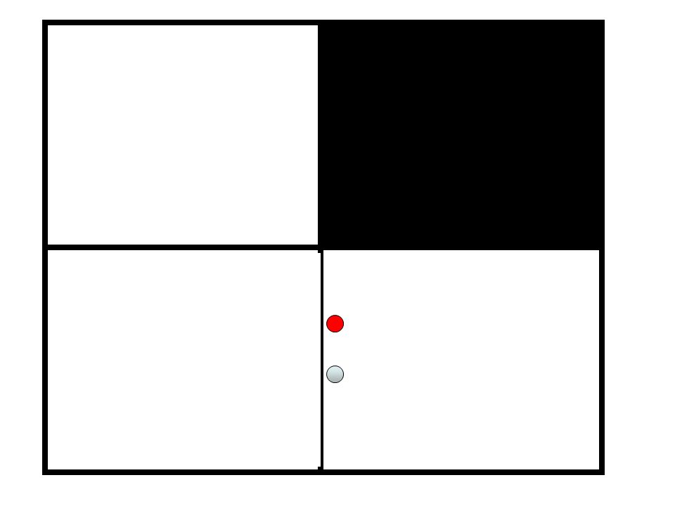
69. A A A A Growth stops when A jumps again (typically after each time interval 1/D A )

70. A A A AA

71. A A AAA

72. A A A Growth stops again when A jumps again (typically after each time interval 1/D A ) A

73. A A A If the time interval d/D A is small, when A jumps back it still finds B ’ s to proliferate A

74. TIME S P C A E ln b TIME (A location and b distribution ) The strict adherence of the elementary particles A and B to the basic fundamental laws and the emergence of complex adaptive entities with self-serving behavior do not interfere one with another. Yet they determine one another. Emergent Collective Dynamics: B-islands search, follow, adapt to, and exploit fortuitous fluctuations in A density. Is this a mystery? Not in the AB model where all is on the table ! This is in apparent contradiction to the “fundamental laws” where individual B don’t follow anybody

76. Conclusions The classical Logistic systems have very non-trivial predictions when treated correctly as made of discrete individuals We have presented some applications: –The confirmation of the model prediction in the Poland liberalization experiment –The qualitative and quantitative confirmation of the model predictions in the scaling properties of market economy and other logistic systems

77. but for d>2 P d (  ) < 1; P 3 (  ) = 0.3405373 Pólya 's Random Walk Constant What is the probability P d (  ) that eventually an A returns to its site of origin? Pólya : P 1 (  ) = P 2 (  ) =1 using it Kesten and Sidoravicius studied the AB model (preprint 75 p): On large enough 2 dimensional surfaces ,  D b  D a  a 0 Total/average B population always grows.

78. Study the effect of one A on b(x,t) on its site of origin x Typical duration of an A visit: 1/D a Average increase of b(x,t) per A visit: e / D a Probability of one A return by time t (d-dimesional grid):P d (t) Expected increase in b(x,t) due to 1 return events: e / D a P d (t) Ignore for the moment the death and emigration and other A’s

79. But for d= 2 P d (  ) =1 so e / D a P d (  ) > 1 e /D a P d (  ) 1 t e / D a P d (t) ee   /2D a > 0   e D a /   <  finite positive expected growth in finite time ! Study the effect of one A on b(x,t) on its site of origin x Typical duration of an A visit: 1/D a Average increase of b(x,t) per A visit: e / D a Probability of one A return by time t (d-dimesional grid):P d (t) Expected increase in b(x,t) due to 1 return events: e / D a P d (t) Ignore for the moment the death and emigration and other A’s

80. { Probability of n returns before time t = n  } > P n d (  ) Growth induced by such an event: e n / D a Expected factor to b(x,t) due to n return events: > [ e / D a P d (  )] n = e n  = e   t   exponential time growth ! -increase is expected at all x’s where: a(x,0) > (  +D b )   There is a finite density of such a(x,0) ’s =>   Taking in account death rate   emigration rate D b and that there are a(x,0) such A’s: > b(x,0) e - (  +D b ) t e a(x,0)  t  

81. Other regimes / mechanisms for island emergence and survival

82. Proliferation and competition in discrete biological systems. Louzoun, Y., Atlan, H., Solomon. S., Cohen, I.R (2003) Bulletin of mathematical biology 65(3) 375-396

105. Directed percolation

106. TIME

107. Directed Percolation TIME

108. Directed Percolation TIME

109. Directed Percolation TIME

110. Directed Percolation TIME

111. Directed Percolation TIME

112. Directed Percolation TIME

113. Other way to estimate finite size effects : Renormalization Group Analysis For more details see: Reaction-Diffusion Systems with Discrete Reactants, Eldad Bettelheim, MSc Thesis, Hebrew University of Jerusalem 2001 http://racah.fiz.huji.ac.il/~eldadb/masters/masters2.html

114. DivisionRate =  Each point represents another AB system: the coordinates represent its parameters: naive effective B decay rate (  - a 0 ) and B division rate B Death Life; Positive Naïve Effective B decay rate = (  - a 0 ) Negative Decay Rate = Growth

115. Each point represents another AB system: the coordinates represent its parameters: naive effective B decay rate (  - a 0 ) and B division rate B Death Life; Positive Naïve Effective B decay rate = (  - a 0 ) Negative Decay Rate = Growth Initially, at small scales, B effective decay rate increases 2  (d-2) D DivisionRate =  Life Wins ! At larger scales B effective decay rate decreases

116. (  - a 0 )

117. (  - a 0 )

118. (  - a 0 )

119. ln size Space / world realization 1 x 10 10 3 x 10 10 9 x 10 10 27 x 10 10

120. Space / world realization ln size 1 x 10 10 3 x 10 10 9 x 10 10 27 x 10 10

121. ln size Space / world realization 1 x 10 10 3 x 10 10 9 x 10 10 27 x 10 10

122. ln size Space / world realization 1 x 10 10 3 x 10 10 9 x 10 10 27 x 10 10

123. ln size Space / world realization 1 x 10 10 3 x 10 10 9 x 10 10 27 x 10 10

124. ln size Space / world realization 1 x 10 10 3 x 10 10 9 x 10 10 27 x 10 10

125. On large enough 2 dimensional surfaces with exceedingly small birth rate and A-density and exceedingly high death rate Life always wins for any A configuration but never at your location at all locations in statistical average (over all A configurations) but never in your particular stochastic realization.

127. EXAMPLE of Theory Application APPLICATION: Liberalization Experiment Poland Economy after 1989 + MICRO growth ___________________ => MACRO growth 1990 MACRO decay (90) 1992 MACRO growth (92) 1991 MICRO growth (91) GNP 89909192 THEOREM (RG, RW) one of the fundamental laws of complexity Global analysis prediction Complexity prediction Education 88 MACRO decay Maps Andrzej Nowak ’ s group (Warsaw U.), CO 3 collaboration